Exponential functions

Section 2.8 Exponential functions

Objectives

Discover how exponential functions can describe percent growth or decay.
🔗

🔗
Learn the definition of exponential functions.
🔗

🔗
Find the formula for an exponential function given two points on the graph of the function.
🔗

🔗
Understand how the values of the coefficient and base of an exponential function affect the shape of the graph.
🔗

🔗

Subsection Motivating exponential functions

When deciding how to model a quantity $q$ as a function of $q=f(a)$ of some other quantity $a\text{,}$ our choice of function is governed by how the output quantity $q$ changes as the input quantity $a$ changes. Recall that the instantaneous rate of change of a function $q=f(a)$ at a specific input $a$ is given by the derivative $f'(a)\text{;}$ and that the derivative $f'(a)$ can be estimated by computing average rates of change over small intervals about $a\text{.}$

🔗

We can distinguish between different types of functions by examining their rate of change at different inputs. For example, the rate of change of a constant functions $f(x)=c$ is zero everywhere, reflecting the fact that the output value of a constant function never changes! Similarly, a linear function $f(x)=ax+b$ has constant rate of change $f'(x)=a\text{,}$ and a quadratic function $f(x)=ax^2+bx+c$ has a linear rate of change function $f'(x)=2ax+b\text{.}$

🔗

In this section we will define and start to explore exponential functions. These functions exhibit a fundamentally different kind of rate of change behavior that also happens to be ubiquitous in real-world empirical phenomena, making them exceptionally useful for modeling purposes.

🔗

Example 2.8.1. Motivating example: percent rate of change.

Suppose that a credit card company is offering a $10\%$ annual interest rate on a one-time loan. If you take out a loan for $\$100$ and don’t make any payments, after one year you still owe the original $\$100\text{,}$ plus 10% of $\$100\text{,}$ so your balance after a year is:

\begin{equation*} 100+0.1(100) = 100+(1+0.01) = 100(1.1)\text{.} \end{equation*}

If we instead borrowed $\$100,000\text{,}$ after 1 year we again owe the original $\$100,000\text{,}$ but now we also owe 10% of $\$100,000\text{,}$ and thus the balance after a year is:

\begin{equation*} 100000+0.1(100000) = 100000(1.1)\text{.} \end{equation*}

If we were to borrow $P$ dollars, we reason the same way that after a year the balance on the loan is

\begin{equation*} P+0.1P = P(1.1) \end{equation*}

🔗

If we go another year without paying anything toward the loan, we repeat our calculations for a second year. Let’s diagram out what happens over two years if we borrow $100$ dollars initially.

🔗

Start	After first year	After second year
$100$	$100(1.1)$	$100(1.1)(1.1) = 100(1.1)^2$

If we started by borrowing $\$100,000\text{,}$ the sequence of debts would be as described below.

🔗

Start	After first year	After second year
$100000$	$100000(1.1)$	$100000(1.1)(1.1) = 100000(1.1)^2$

Using the same reasoning, if we borrow $P$ dollars without paying anything back, the sequence of debts over two years follows the same pattern.

🔗

Start	After first year	After second year
$P$	$P(1.1)$	$P(1.1)(1.1) = P(1.1)^2$

What will happen after 3 years? Adding $10\%$ to the loan balance of $P(1.1)^2$ after two years, the original loan $P$ will have grown to

\begin{equation*} P(1.1)^3\text{.} \end{equation*}

🔗

Here we see a new kind of pattern developing: annual growth of $10\%$ is leading to powers of the base $1.1\text{,}$ where the power to which we raise $1.1$ corresponds to the number of years the loan has grown. Note that the change occurs in the exponent of the formula:

\begin{equation*} P(1.1)^t \end{equation*}

where $t$ is the number of years since we took out the loan. Each additional year results in an additional multiplication by $1.1\text{,}$ so for each year that passes, the power of the base $1.1$ will increase by $1\text{.}$ This type of change is an example of exponential growth.

🔗

Subsection Defining Exponential Functions

The pattern described by the example above is new to us. We have yet to see a function where the variable is in the exponent. It turns out that such functions are not algebraic, although proving this to be the case is not straightforward. We call a function transcendental if it is not algebraic. In this course we will eventually introduce four different types of transcendental functions: exponential, logarithmic, trigonometric, and inverse trigonometric functions. We begin with exponential functions, which we will now endeavor to define as best we can. Exponential functions look similar to power functions, but with the roles of constant and variable reversed in the base and exponent.

🔗

Definition 2.8.2. Exponential Functions.

An exponential function is a function $f\colon \R\rightarrow \R$ that can be written in the form

\begin{equation*} f(x) = Ab^x \end{equation*}

for some real numbers $A$ and $b$ such that $A\neq 0, b> 0\text{,}$ and $b\neq 1\text{.}$

🔗

Remark 2.8.3. Power functions versus exponential functions.

It is easy to conflate a power functions $f(x)=cx^k$ with an exponential function $g(x)=Ab^x\text{,}$ since both are defined using the power operation. The key difference between the two types of functions is the precise position of the input variable $x\text{:}$

in a power function $f(x)=cx^k\text{,}$ the input variable $x$ appears as the base of the power expression;
🔗

🔗
in an exponential function $g(x)=Ab^x\text{,}$ the input variable $x$ appears as the exponent of the power expression. Hence the name.
🔗

🔗

🔗

Remark 2.8.4. Domain of exponential function.

As defined, the domain of an exponential function $f(x)=A b^x$ is $\R\text{,}$ the set of all real numbers. The conscientious reader may object, however, that when defining power expressions like $b^x\text{,}$ we only did so for rational exponents of the form $x=m/n\text{,}$ where $m$ and $n$ are integers. For example, we have given no definition of the power expression $3^{\sqrt{2}}\text{.}$ To that conscientious reader we say: you are absolutely justified! Of course there is a perfectly rigorous way to define $b^x$ for all $x\in \R$ (not just rational $x$), but for now you will just have to take this on faith. For the time being, we are more focused on detailing the important properties of exponetial functions so that you can make use of them in modeling situations.

🔗

Since exponential functions involve a power expression of the form $a^b\text{,}$ you in order to facilitate working with them, you may want to review the various rules governing power expressions articulated in Theorem 1.4.5. The next example illustrates how these can be put to use.

🔗

Example 2.8.5. Standard form of exponential functions.

Each function below is exponential. Write it in the standard form $f(x)=Ab^x\text{.}$

$\displaystyle f(x)=3\cdot 2^{2x}$
🔗

🔗
$\displaystyle f(x)=\dfrac{4}{5\cdot 3^{x}}$
🔗

🔗
$\displaystyle f(x)=6^{x/5}$
🔗

🔗
$\displaystyle f(x)=\sqrt[3]{\dfrac{8^x}{27}}$
🔗

🔗
$\displaystyle f(x)=2^{x-1}$
🔗

🔗

🔗

Solution.

We have

\begin{align*} f(x) \amp = 3\cdot 2^{4x}\\ \amp =3\cdot (2^4)^x\\ \amp =3\cdot 16^x\text{.} \end{align*}

🔗

🔗
We have

\begin{align*} f(x) \amp = \dfrac{4}{5\cdot 3^{x}}\\ \amp = \dfrac{4}{5}\cdot 3^{-x}\\ \amp = \dfrac{4}{5}(3^{-1})^x\\ \amp = \dfrac{4}{5}\cdot \left(\dfrac{1}{3}\right)^x\text{.} \end{align*}

🔗

🔗
We have

\begin{align*} f(x) \amp = 6^{x/5}\\ \amp = (6^{1/5})^x\text{.} \end{align*}

🔗

🔗
We have

\begin{align*} f(x) \amp = \sqrt[3]{\dfrac{8^x}{27}}\\ \amp = \left(\dfrac{8^x}{27}\right)^{1/3}\\ \amp = \dfrac{(8^x)^{1/3}}{27^{1/3}}\\ \amp = \dfrac{8^{x/3}}{3}\\ \amp = \dfrac{1}{3}\cdot (8^{1/3})^x\\ \amp = \dfrac{1}{3}\cdot 2^x\text{.} \end{align*}

🔗

🔗
We have

\begin{align*} f(x) \amp = 2^{x-1}\\ \amp = 2^x\cdot 2^{-1}\\ \amp = \dfrac{1}{2}\cdot 2^x\text{.} \end{align*}

🔗

🔗

🔗

Subsection Growth of exponential Functions

Let’s look at another practical application of exponential functions in order to better understand their properties:

🔗

Example 2.8.6.

Suppose that at age 25 you receive a signing bonus of $20,000 at your new job

Congratulations!

and you can choose between one of two ways to use the money: you can invest it in a mutual fund that will, on average, earn 8% interest annually, or you can purchase a used car that will, on average, depreciate 12% annually. Let’s explore how the $20,000 changes over time.

🔗

Let $M(t)$ denote the value of the $20,000 after $t$ years if it is invested in the mutual fund. Let $C(t)$ denote the value of the car $t$ years after it is purchased.

🔗

We know that $M(0)=20000$ since when $t=0\text{,}$ you are starting with $20,000. After one year you will have 8% more, so that

\begin{equation*} M(1) = 20000+0.8(20000) = 20000(1.08) = 21600\text{.} \end{equation*}

🔗

In general, a quantity increasing by 8% annually will be multiplied by 1.08 each year, so that

\begin{equation*} M(2) = 20000(1.08)^2 = 23,328\qquad\text{ and } \qquad M(3) = 20000(1.08)^3 = 25194.24\text{.} \end{equation*}

🔗

A formula for $M(t)$ after $t$ years is then

\begin{equation*} M(t) = 20000(1.08)^t\text{.} \end{equation*}

A graph of $M(t)$ is

🔗

Figure 2.8.7. $M(t) = 20000(1.08)^t$ describes 8% annual growth over $t$ years.
🔗

Let’s now look at the value of the car. We know that $C(0) = 20000\text{.}$ After one year, the value of the car will be 12% less than it was originally worth, so that

\begin{equation*} C(1) = 20000-0.12(20000) = 20000(1-0.12) = 20000(0.88)= 17600\text{.} \end{equation*}

🔗

Note that if a quantity depreciates (meaning decreases by) 12% annually, after a given year, $(100-12)\% = 88\%$ of that quantity remains. So for each year that passes, we multiply by another $0.88\text{:}$

\begin{equation*} C(2) =20000(0.88)^2= 15488\qquad\text{ and } \qquad C(3) = 20000(0.88)^3= 13629.44\text{.} \end{equation*}

🔗

A formula for $C(t)$ after $t$ years is then

\begin{equation*} C(t) = 20000(0.88)^t\text{.} \end{equation*}

A graph of $C(t)$ is

🔗

Figure 2.8.8. $C(t) = 20000(0.88)^t$ describes 12% annual depreciation over $t$ years.
🔗

🔗

Note the very different behavior of the two functions: 8% growth results in an increasing, concave up function, while 12% depreciation results in a decreasing, concave up function. Both functions have a coefficient of $A=20000\text{.}$ The only difference in the formula is in the base $b$ of the exponential function: growth corresponds to a base of $b=1.08>1\text{,}$ while depreciation corresponds to a base of $b=0.88\lt 1\text{.}$ This is not a coincidence. Bases larger than 1 will increase as the exponent increases, while bases between 0 and 1 will decrease as the exponent increases.

🔗

For an exponential function $f(x)=Ab^x\text{,}$ we note that $f(0) = A\cdot b^0 = A\cdot 1 = A\text{,}$ so an exponential function has $y$-intercept equal to the coefficient $A\text{.}$ This is sometimes called the initial value of the quantity being modeled. In the example above, $M(0) = 20000$ and $C(0)=20000$ are the initial quantity of your bonus that you either invested or paid for the car.

🔗

Note that because a positive number raised to any power is always positive (for instance, $2^{10} = 1024$ and $2^{-10} = \frac{1}{2^{10}} = \frac{1}{1024}$), the expression $b^x$ is also always positive. An exponential function $f(x) = Ab^x$ will then always be positive when the coefficient $A$ is positive and will always be negative when $A$ is negative. In particular, $f(x) = Ab^x$ is never zero, and thus has no $x$-intercepts. In the example above, $M(t)$ and $C(t)$ both have positive coefficient $A=20000\text{,}$ so these two quantities will always be positive for any value of $t\text{.}$ This makes sense intuitively in both examples: the values of the mutual fund and car cannot be negative.

🔗

Again looking at Example 2.8.6, we call $1.08$ the "growth factor" of $M$ and similarly $0.88$ the growth factor of $C$ because we are multiplying by that factor for each 1-unit increase in time. In addition, we note that these values stem from the actual growth rates: $8\% = 0.08$ for $M\text{,}$ so that the growth factor is $1+0.08\text{,}$ and $-12\% = -0.12$ for $C\text{,}$ so that the growth factor is $1-0.12\text{,}$ the latter growth rate being negative because value is deprecating. In general, for a function of the form $f(x) = Ab^x\text{,}$ we call $b$ the growth factor. Moreover, if $b = 1+r\text{,}$ we call $r$ the growth rate. Whenever $b> 1\text{,}$ we often say that the function $f$ is exhibiting exponential growth, whereas if $0\lt b\lt 1\text{,}$ we say $f$ exhibits exponential decay.

🔗

Checkpoint 2.8.9.

In your own words, explain the difference between growth factor and growth rate. Use the context of Example 2.8.6 to help you explain.

🔗

Let’s compare linear and exponential functions to best illustrate this new growth pattern.

🔗

Example 2.8.10. Growth patters: linear versus exponential Functions.

In the tables below, we see output for two different functions $r$ and $s$ that correspond to equally spaced inputs:

🔗

$t$	0	3	6	9

$r(t)$	12	10	8	6

Table 2.8.11. Table of values for $r(t)$

🔗

$t$	0	3	6	9

$s(t)$	12	9	6.75	5.0625

Table 2.8.12. Table of values for $s(t)$

🔗

In the left-hand table, we see a function that exhibits constant average rate of change since the change in output is always $\Delta r = -2$ for any change in input of $\Delta t = 3\text{.}$ Said differently, $r$ is a linear function with slope

\begin{equation*} m =\frac{\Delta r}{\Delta t} = -\frac{2}{3}\text{.} \end{equation*}

Since its $y$-intercept is $(0,12)\text{,}$ the function’s formula is

\begin{equation*} y=r(t) = -\frac{2}{3}t+12\text{.} \end{equation*}

🔗

The difference between one output and the next is always a constant $-2\text{,}$ as long as the input increases by 3.

🔗

By contrast, the function $s$ given by the right-hand table does not exhibit constant average rate of change:

\begin{equation*} AV_{[0,3]} = \frac{9-12}{3-0} = -1, AV_{[3,6]} = \frac{6.75-9}{6-3} = -0.75, AV_{[6,9]} = \frac{5.0625-6.75}{9-6} = -0.5625\text{.} \end{equation*}

🔗

Thus the difference between one output and the next is not constant as the input increases by a constant amount and $s(t)$ is not a linear function.

🔗

Instead, observe that in the table for $s(t)\text{,}$ each output is a multiple of the previous output. The first two outputs have a ratio of

\begin{equation*} \frac{9}{12} = \frac{3}{4}\text{.} \end{equation*}

The second and third outputs have a ratio of

\begin{equation*} \frac{6.75}{9} = 0.75 = \frac{3}{4} \end{equation*}

🔗

The third and fourth outputs have a ratio of

\begin{equation*} \frac{5.0625}{6.75} = 0.75 = \frac{3}{4}\text{.} \end{equation*}

For $r(t)\text{,}$ we see that when the input increases by 3, the output is multiplied by $\frac{3}{4}\text{.}$ As a formula,

\begin{equation*} s(t) = 12\left(\frac{3}{4}\right)^{t/3} \end{equation*}

🔗

Summarizing the key difference between linear and exponential change:

🔗

\fbox{ Whereas the differences in the outputs of a linear function are constant, the ratios in the outputs of the exponential function are constant (over equally spaced inputs). }

🔗

Checkpoint 2.8.13.

In Example 2.8.10, the exponent of $\frac{3}{4}$ is $t/3\text{.}$ Why does this translate to multiplying by $\frac{3}{4}$ when $t$ increases by $3\text{?}$ What would happen if we used $3t$ as the exponent instead?

🔗

Subsection Finding Formulas for Exponential Functions

We now do some algebra. Recall that we can find the formula of a linear function from knowing only two points that lie on the line. Similarly, if we know two points on the graph of an exponential function, we can determine the function’s formula. We demonstrate two different methods for doing so in the next example and the following exercise.

🔗

Example 2.8.14.

Suppose that $p$ is an exponential function and we know that $p(2)=11$ and $p(5) = 18\text{.}$ Determine the exact values of $A$ and $b$ for which $p(t) = Ab^t\text{.}$

🔗

Solution.

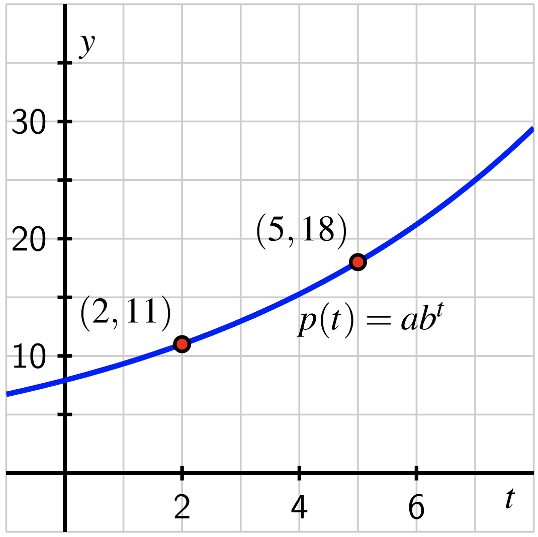
Since we know that $p(t) = Ab^t\text{,}$ the two data points give us two equations in the unknowns $A$ and $b\text{.}$ First, using $t=2\text{,}$

\begin{equation*} Ab^2 = 11\text{,} \end{equation*}

and using $t=5$ we also have

\begin{equation*} Ab^5 = 18\text{.} \end{equation*}

🔗

Because we know that the ratios of outputs of an exponential function corresponding to equally-spaced inputs must be constant, we consider the ratio of our outputs $\frac{18}{11}\text{:}$

\begin{equation*} \frac{18}{11} = \frac{Ab^5}{Ab^2} = \frac{b^5}{b^2} =b^3\text{.} \end{equation*}

🔗

Solving for $b\text{,}$ we find that

\begin{equation*} b = \sqrt[3]{\frac{18}{11}}\approx 1.1784\text{.} \end{equation*}

🔗

Using the exact value $b = \sqrt[3]{\frac{18}{11}}$ and substituting this value for $b$ in $Ab^2 = 11\text{,}$ we see that

\begin{equation*} A\left(\sqrt[3]{\frac{18}{11}}\right)^2 = 11 \Rightarrow A = \frac{11}{\left(\frac{18}{11}\right)^{2/3}}\approx 7.9215 \end{equation*}

🔗

Therefore,

\begin{equation*} p(t) = \frac{11}{\left(\frac{18}{11}\right)^{2/3}}\left(\sqrt[3]{\frac{18}{11}}\right)^t\approx 7.9215(1.1784)^t \end{equation*}

and a plot of $y=p(x)$ confirms that the function indeed passes through $(2,11)$ and $(5,18)\text{:}$

🔗

Checkpoint 2.8.15. Another Approach.

In Example 2.8.14, we saw that as the input $t$ increases by $5-2=3\text{,}$ the ratio of the outputs is $\frac{18}{11}\text{.}$ Since the ratio of outputs is constant for exponential functions, another increase of $3$ in $t$ will result in multiplication by another $\frac{18}{11}\text{,}$ so that

\begin{equation*} p(t) = A\left(\frac{18}{11}\right)^{t/3} \end{equation*}

🔗

From here, use the fact that $p(2)=11$ (or $p(5)=18\text{;}$ you can use either) to find $A\text{.}$ Verify that this value of $A$ is the same as was found in Example 2.8.14. (You will probably want to write what you found as a decimal.)

🔗

Lastly, observe that:

\begin{equation*} \left(\frac{18}{11}\right)^{t/3} = \left(\frac{18}{11}\right)^{(1/3)\cdot t} =\left(\sqrt[3]{\frac{18}{11}}\right)^t \end{equation*}

so that the base of the two functions is the same if we isolate $t$ in the exponent.

🔗

Subsection Properties of Exponential Functions

We’ve seen in our examples so far that exponential function arise when modeling quantities that change by a percent of their value. In this section, we will explore how this affects the shape of such functions.

🔗

Example 2.8.16. Exponential functions: graphical properties.

Use the Desmos interactive in Figure 2.8.17 to answer the following questions.

The Desmos graph is initially set to $A=1$ and $b=2\text{.}$ Describe the shape of the resulting function $f(x) = 2^x\text{.}$ Is the function positive? Negative? Increasing? Decreasing? Concave up? Concave down?
🔗

🔗
Experiment setting $A$ to any nonzero number (try both positive and negative) and setting $b$ to either a number between 0 and 1, or a number greater than 1. How do these different choices affect the shape of the graph?
🔗

🔗
Why can’t we use $A=0\text{?}$ Set $A=0$ in the Desmos graph. How does this change the shape of the graph? Would you call this graph "exponential?"
🔗

🔗
Why can’t we have $b=1\text{?}$ Set $A$ to any nonzero number and $b=1\text{.}$ How does this change the shape of the graph? Would you call this graph "exponential?"
🔗

🔗
Set $b=-0.5\text{.}$ It’s going to look very strange (if Desmos shows you anything; sometimes it doesn’t). Think about what values we can have for the exponent $x$ in the expression $f(x) = A(-0.5)^x\text{.}$ What would happen with $x=\frac{1}{2}\text{?}$ $x=-\frac{1}{4}\text{?}$ $x=\frac{97}{6}\text{?}$ There are infinitely many values of $x$ for which a negative base would result in an undefined expression. This is why the definition of an exponential function excludes $b\lt 0\text{.}$
🔗

🔗

🔗

Figure 2.8.17. Desmos interactive: graphs of exponential functions

🔗

If we consider an exponential function $f$ with a growth factor $b> 1\text{,}$ such as the function pictured to the left below, then the function is always increasing because higher powers of $b$ are greater than lesser powers (for example, $(1.2)^3> (1.2)^2$). On the other hand, if $0\lt b\lt 1\text{,}$ such as the function pictured to the right below, then the exponential function will be decreasing because higher powers of positive numbers less than 1 get smaller (for example, $(0.9)^3\lt (0.9)^2$). If you don’t believe this, plug the numbers into a calculator.

🔗

Exponential growth function — (a) $f(x)=b^x\text{,}$ $b> 1$
🔗

Exponential decay function — (a) $f(x)=b^x\text{,}$ $b> 1$
🔗

We also notice that each graph bends upward and is therefore concave up. We can better understand why this is so by considering the average rate of change of both $f$ and $g$ on consecutive intervals of width 1, so that the average rate of change can be computed by

\begin{equation*} AV_{[t,t+1]} = \frac{f(t+1)-f(t)}{1} = f(t+1)-f(t)\text{.} \end{equation*}

The tables below give the average rate of change of $f(t) = 2(1.25)^t$ and $g(t) = 8(0.75)^t$ on several consecutive unit intervals:

🔗

Figure 2.8.19. Average rate of change of $f(t) = 2(1.25)^t$
🔗

Figure 2.8.20. Average rate of change of $g(t) = 8(0.75)^t$
🔗

The exponential function $f$ in Figure 2.8.19 is seen to have an average rate of change that is positive and increasing. This suggests that $f$ is increasing at an increasing rate. As a result, the graph of $f$ is concave up.

🔗

Similarly, the exponential function $g$ in Figure 2.8.20 is seen to have an average rate of change that is negative but increasing (getting less negative). This suggests that $g$ is decreasing at a decreasing rate. As a result, the graph of $g$ is also concave up.

🔗

We summarize a few of these observations here:

🔗

Theorem 2.8.21. Properties of Exponential Functions.

For an exponential function of the form $f(x) = Ab^x$ where $A$ and $b$ are both positive with $b\neq 1\text{,}$

The value of $f(x)$ is never zero for any $x\in\mathbb{R}\text{.}$
🔗

🔗
If $b> 1\text{,}$ then $f$ is always increasing and concave up.
🔗

🔗
If $0\lt b\lt 1\text{,}$ then $f$ is always decreasing and concave up.
🔗

🔗
The graph of $f$ passes the Horizontal Line Test.
🔗

🔗

🔗

Note the last statement: the graph of $f$ passes the Horizontal Line Test. This is because $f$ is either increasing or decreasing and so its graph cannot repeat values. Another way to say this is that exponential functions are one-to-one and that every exponential function has an inverse! Let’s repeat that:

🔗

\fbox{ Every exponential function has an inverse!!! }

🔗

In the next section, we will define and explore the inverses of exponential functions. They are called logarithms.

🔗

Checkpoint 2.8.22.

Since exponential functions are one-to-one, if $b^c = b^d\text{,}$ then we must have $c=d\text{.}$ Use this property to determine the value of $x$ that satisfies each equation below. This will be useful in the next section when we want to find values of logarithms.

Find $x$ with $2^x = 8$ by rewriting $8$ as a power of $2\text{.}$
🔗

🔗
Find $x$ with $3^x = \frac{1}{81}$ by rewriting $\frac{1}{81}$ as a power of $3\text{.}$
🔗

🔗
Find $x$ with $\left(\frac{1}{25}\right)^x = 125$ by rewriting $\frac{1}{25}$ and $125$ as powers of $5\text{.}$
🔗

🔗

🔗

Prev Top Next

\(t\)	0	3	6	9

\(r(t)\)	12	10	8	6

\(t\)	0	3	6	9

\(s(t)\)	12	9	6.75	5.0625