A function is a fundamental mathematical object that will form the basis of everything we study in this course. In this section, we will explore their definition and its meaning, several ways of representing a function, and a physical example of how functions are manifest in real-world phenomena.
If you look up "function" in the Merriam-Webster dictionary (click on this link: https://www.merriam-webster.com/dictionary/function), there are many different meanings. Which ones agree with the ideas you already had? The fifth entry 1
Part (a) of this definition is the abstracted, theoretical idea of a function. Part (b) of this definition is the reason we are interested in functions: we wish to describe relationships between real-world quantities. We will begin with the abstract idea before applying this knowledge to something more concrete.
In Definition 1.1.3 we give a formal, mathematical statement that we shall take to be the precise meaning of the word “function”. Return to this definition as you read the examples that follow in order to make sense of the notation and terminology.
To make our definition as rigorous as possible, we will make use of some notions and notation related to the mathematical theory of sets that we now officially introduce.
A set \(A\) is a collection of objects, called the members or elements of \(A\text{.}\) We write \(a\in A\) if the object \(a\) is a member of \(A\text{,}\) and \(a\notin A\) if \(a\) is not a member of \(A\text{.}\)
is a rule which, given any input \(a\in A\text{,}\) returns a unique output \(b\in B\text{.}\) We write \(b=f(a)\) in this case, and call \(b\) the image of \(a\) under \(f\text{,}\) or the value of \(f\) at \(a\text{.}\) Similarly, we say \(f\) maps (or sends) the input \(a\) to the output \(b=f(a)\text{.}\)
The essential detail in the definition of a function \(f\colon A\rightarrow B\text{,}\) is that for each input \(a\) in our domain \(A\) the functions assigns a unique output \(b\) in our codomain \(B\text{.}\) This detail introduces a fundamental asymmetry between the roles of the variable \(a\) and the variable \(b\) in the context of the function \(f\colon A\rightarrow B\text{.}\) We codify this asymmetry with the terms independent variable and dependent variable.
In more detail, we call the variable \(a\text{,}\) which is allowed to range freely over all elements of the domain \(A\text{,}\) an independent variable of \(f\text{;}\) and we call the variable \(b\) a dependent variable of \(f\text{,}\) as given any input \(a\text{,}\) the output \(b=f(a)\) is determined by \(a\text{.}\)
Consider the rule \(f\) that takes as input any real number and returns as an output the square of that number. This rule defines a function since for any real number \(x\text{,}\) its square \(x^2=x\cdot x\) is uniquely determined.
Let’s flesh out all the details of the function \(f\text{,}\) as well as the accompanying notation. Observe that the phrase “takes as input any real number” implies that the domain of \(f\) is \(\R\text{,}\) the set of all real numbers. Since the square of a real number is itself a real number, we see that we can also set our codomain to be \(\R\text{.}\)
Letting \(x\) and \(y\) denote the independent and dependent variables of \(f\text{,}\) respectively, we write \(y=x^2\) or \(y=f(x)\) to represent the fact that the values of \(y\) are the result of squaring \(x\text{,}\) or equivalently, applying the function \(f\) to \(x\text{.}\)
Using the language of Definition 1.1.3, this means that the value of \(f\) at \(3\) is \(9\text{,}\) and the value of \(f\) at \(-3\) is also \(9\) (or alternatively, \(f\) maps both \(3\) and \(-3\) to the output \(9\)).
from Example 1.1.5 nicely illustrate the asymmetry in the roles of independent variable and dependent variable mentioned in Remark 1.1.4. Whereas, by definition, corresponding to each input of a function there is a unique output, it is not necessarily the case that for each output of the function there is a unique input that gets mapped to it. In this case, we see that the output \(y=9\) is the value of \(f\) at two different inputs: \(x=3\) and \(x=-3\text{.}\) More on this later, when we discuss invertible functions.
Intimately related to the squaring operation on \(\R\) is the notion of square roots. Recall that given a real number \(x\in \R\text{,}\) a (real) square root of \(x\) is a number \(y\in \R\) satisfying \(y^2=x\text{.}\) For example, \(2\) is a square root of \(4\text{,}\) since \(2^2=4\text{.}\) It is possible to define a function based on square roots, but we have to proceed with caution, as the next example illustrates.
Explain why the following proposed rule does not define a function \(f\colon \R\rightarrow \R\text{:}\) given a real number \(x\in \R\text{,}\) define \(f(x)\) to be the square root of \(x\text{.}\)
Firstly, not every real number \(x\) has a (real) square root! Consider \(x=-1\text{,}\) for example. We cannot have \(-1=y^2\) for a real number \(y\in \R\) since \(y^2\geq 0\) for any \(y\in \R\) and \(-1< 0\text{.}\) More generally, no negative real number has a square root.
The specific issue described in (1) is easily remedied by replacing our domain \(\R\) with the smaller domain \(D\) of all nonnegative numbers \(x\geq 0\text{,}\) since it is a (nontrivial) fact that every nonnegative real number has a square root. However, a separate issue arises preventing \(f\) from being a well-defined function. Namely, with the exception of \(x=0\text{,}\) a nonnegative number has two distinct square roots. For example, the number \(x=4\) has two square roots: \(y=2\) and \(y=-2\text{.}\) This means there is no such thing as “the” square root, even if we restrict our attention to nonnegative numbers! Since our rule fails to assign a unique output for each input of the domain, it fails to be a function.
Our discussion of Example 1.1.7 laid bare two issues that arise when defining a function that computes square roots: (1) not all real numbers have a square root; and (2) positive real numbers have two distinct square roots (if \(y\) is a square root of \(x\text{,}\) then so is \(-y\)). The principal square root function defined in Definition 1.1.8 sorts these issues out by taking as its domain the set of all nonnegative real numbers (since nonnegative numbers do have square roots) and choosing for each nonnegative integer its unique nonnegative square root (only one of \(y\) and \(-y\) will be nonnegative).
Given any nonnegative real number \(x\geq 0\text{,}\) we denote by \(\sqrt{x}\) its unique nonnegative square root, and we call \(\sqrt{x}\) the principal square root of \(x\) (or more casually, the radical of \(x\)).
Let \(D\) be the set of all nonnegative real numbers \(x\geq 0\text{.}\) The function \(f\colon D\rightarrow \R\) defined as \(f(x)=\sqrt{x}\) is called the principal square root function.
Texts (and instructors) can be pretty sloppy when dealing with the principal square root operation, often referring to the expression \(\sqrt{x}\) as “the square root of \(x\)”. This seemingly innocuous mistake can lead to larger misconceptions down the line. As such you are encouraged to adopt the following habit: each time you see \(\sqrt{x}\) utter to yourself “the nonnegative square root of \(x\)”.
What are two other examples of functions that you can think of? These may be mathematical examples that you have seen before, or they may be real-world examples of a quantity that varies depending on another. Try to be creative!
In order to describe the domains, codomains, and ranges (see Definition 1.1.22 below) of functions we will need some more set theory concepts and notation.
A set \(A\) is a subset of a set \(B\text{,}\) denoted \(A \subseteq B\text{,}\) if every member of \(A\) is a member of \(B\text{:}\) i.e., \(a\in A\) implies \(a\in B\text{.}\) The relation \(A\subseteq B\) is called set inclusion.
Let \(A\) be a set, and let \(P\) be a property that elements of \(A\) either satisfy or do not satisfy. For an element \(a\in A\text{,}\) let \(P(a)\) denote the statement that \(a\) satisfies property \(P\text{.}\) The set of all elements of \(A\) that satisfy property \(P\) is denoted
\begin{equation*}
\{a \in A \mid P(a) \}\text{.}
\end{equation*}
Set-builder notation is a convenient means of carving out an interesting subset from an existing set using a defining property. For example, the set \(D\) of all nonnegative real numbers, which appeared as the domain of the principal square root function, can be described using set-builder notation as
Using Definition 1.1.12, we see that \(A\) is the set of integers satisfying the property of being greater than 0. In other words, \(A\) is precisely the set of positive integers. We can describe \(A\) enumeratively as
Again following Definition 1.1.12, we see that \(B\) is the set of all integers satisfying the property that they are equal to \(2k\) for some integer \(k\text{.}\) Said another way, \(B\) is the set of integers that are multiples of \(2\text{.}\) Such integers are called even, and we conclude that \(B\) is the set of all even integers. We can enumerate \(B\) as
When dealing with subsets of \(\R\) it is often convenient to make use of interval notation. Intervals are special types of subsets of \(\R\text{.}\) Roughly speaking, for a subset \(I\) of \(\R\) to be an interval means that if \(I\) contains two elements \(x\) and \(y\text{,}\) then it also contains all real numbers between\(x\) an \(y\text{.}\) The set
Instead of burdening you with a formal definition of intervals, we simply provide in Table 1.1.15 examples of various kinds of intervals. In that table \(a\) and \(b\) are assumed to be real numbers satisfying \(a< b\text{.}\)
Note that, roughly speaking, a square bracket ([ and ] ) indicates the inclusion of the corresponding number in the interval, whereas a parenthesis indicates that the number is excluded. Graphically speaking a number being included or excluded from the interval is indicated by either a closed (solid) or open dot, respectively.
Let \(A\) and \(B\) be subsets of a common set \(X\text{.}\)
The union of \(A\) and \(B\text{,}\) denoted \(A\cup B\) is defined as the set of all elements of \(X\) that lie either in \(A\) or \(B\text{:}\) i.e.,
\begin{equation*}
A\cup B=\{x\in X\mid x\in A \text{ or } x\in B\}\text{.}
\end{equation*}
The intersection of \(A\) and \(B\text{,}\) denoted \(A\cap B\) is defined as the set of all elements of \(X\) that lie both in \(A\) and \(B\text{:}\) i.e.,
\begin{equation*}
A\cap B=\{x\in X\mid x\in A \text{ and } x\in B\}\text{.}
\end{equation*}
For an element \(x\in \R\) to not be in \([1,2]\) is equivalent to \(x\) either being less than \(1\) or greater than \(2\text{:}\) i.e., we have \(x\in (-\infty, 1)\) or \(x\in (2,\infty)\text{.}\) Thus we have
At this point we have introduced a number of important sets and their corresponding notation. Let’s make these official with a definition. We also take the opportunity to add one more important set to our repertoire: the empty set.
According to Definition 1.1.3, to give a complete definition of a function, we need to specify three things: the domain of the function, its codomain, and the rule that defines the value of the function at each of its inputs. Consequently, a statement like
\begin{equation}
\text{ let } f(x)=x^2\tag{1.5}
\end{equation}
is technically speaking not a complete definition of a function, since it does not specify the domain and codomain in question. So as not to get bogged down by such technicalities, we hereby adopt the following convention in the form of an official decree, or fiat.
If a function \(f\) is introduced via a formula without specifying a domain or codomain, we will assume that the codomain is \(\R\) and that the implied domain \(D\) is the set of all real numbers for which the formula can be meaningfully evaluated.
Let \(f\) be the function defined as \(f(x)=1/x\text{.}\) Following Fiat 1.1.20, give a full definition of this function by determining the codomain and implied domain. Use interval notation to describe these sets.
Since \(f\) is only given as a formula, following Fiat 1.1.20, the codomain of \(f\) is \(\R=(-\infty, \infty)\) and the implied domain is the set of all real numbers \(x\) for which the formula \(1/x\) makes sense. Since the fraction \(1/x\) is well-defined if and only of \(x\ne 0\text{,}\) we conclude that the domain \(D\) of \(f\) is the set of all nonzero real numbers: i.e.,
In addition to the domain and codomain of a function, another important set associated to it is the set of all possible outputs. Consider again the function \(f(x)=x^2\text{,}\) whose domain and codomain, following Fiat 1.1.20, are both equal to \(\R\text{.}\) You may recall, however, that squares of real numbers are in fact nonnegative real numbers: i.e., \(x^2\geq 0\) for all \(x\in \R\text{.}\) This means that the set of outputs of \(f\colon \R\rightarrow \R\) is strictly smaller than the codomain \(\R\) as it does not contain any negative real numbers. There is nothing wrong with this. In general, the codomain of a function should be thought of simply as a target set that the outputs of \(f\) land in; our function definition Definition 1.1.3 does not insist that every element of the codomain must be an output of the function. That said, the set of all outputs of a function is important to us, and as such warrants an official name: the range of the function.
The range of a function \(f\colon A\rightarrow B\text{,}\) denoted \(\range f\text{,}\) is the set of all outputs of \(f\text{.}\) Using set-builder notation, we have
\begin{equation}
\range f=\{b\in B\colon b=f(a) \text{ for some } a\in A\}\text{,}\tag{1.6}
\end{equation}
Note that the definition of the range of a function \(f\colon A\rightarrow B\) depends very much on the domain \(A\text{,}\) since it is the set of all outputs of the form \(f(a)\text{,}\) where \(a\in A\text{.}\) This is one reason why when defining a function we must know precisely what the domain is.
For example consider the two following functions: \(f\colon \R\rightarrow \R \text{,}\)\(f(x)=2x\text{;}\)\(g\colon [1,\infty)\rightarrow \R\text{,}\)\(g(x)=2x\text{.}\) Although the functions are defined using the same rule, since they have different domains, they are strictly speaking different functions. This difference is reflected in their having different ranges. Indeed, an argument along the lines of the ones given in Example 1.1.24 and Example 1.1.25 reveals that
\begin{align*}
\range f \amp =\{2x\colon x\in \R\}=\R\\
\range g \amp =\{2x\colon x\in [1,\infty)\}=[2,\infty)\text{.}
\end{align*}
As a result, when computing the range of a function, it is absolutely essential to know precisely what the domain of the function is.
First we apply Fiat 1.1.20 to determine the codomain and implied domain of \(f\text{.}\) As always in this setting, the codomain is \(\R\text{.}\) Furthermore, since the defining expression \(x^2\) of \(f\) makes sense for any real number, we conclude that the domain of \(f\) is \(\R\) and we write \(f\colon \R\rightarrow \R\text{.}\)
\begin{align*}
\range f \amp =\{y\in \R\mid y=f(x) \text{ for some } x\in \R\}\\
\amp = \{y\in \R\mid y=x^2 \text{ for some } x\in \R\}\\
\amp = \{x^2\mid x\in \R\}\text{.}
\end{align*}
Since \(x^2\geq 0\) for all \(x\in \R\text{,}\) and since every element of \(\range f\) is of the form \(x^2\) for some \(x\text{,}\) we see that all elements of \(\range f\) are nonnegative, and hence that \(\range f\subseteq [0,\infty)\text{.}\) As you might have guessed, this set inclusion is in fact an equality: i.e., we claim that \(\range f=[0,\infty)\text{.}\)
To prove this claim, it remains only to show the reverse set inclusion: i.e., that every nonnegative real number \(y\geq 0\) is an element of \(range f\text{,}\) or equivalently, that if \(y\geq 0\text{,}\) then we have \(y=f(x)=x^2\) for some \(x\in \R\text{.}\) This in turn is equivalent to showing that if \(y\geq 0\text{,}\) then we can solve the equation
\begin{equation}
y=x^2\tag{1.8}
\end{equation}
for \(x\text{.}\) Thankfully, this is not so difficult. Indeed, given any \(y\geq 0\text{,}\) the number \(x=\sqrt{y}\) satisfies \(x^2=(\sqrt{y})^2=y\text{.}\) (Of course, \(x=-\sqrt{y}\) is another solution to (1.8), but we only needed to provide one.) Putting it all together, we conclude that given any \(y\geq 0\text{,}\) we have \(y=f(x)\text{,}\) where \(x=\sqrt{y}\text{.}\) This shows that every nonnegative real number is an element of \(\range f\text{,}\) and completes the proof that
Firstly, we observe that the implied domain of \(f\) is \(D=[0,\infty)\text{,}\) since the expression \(\sqrt{x}\) is only defined for nonnegative real numbers \(x\text{.}\) We claim that
Indeed, since by definition \(\sqrt{x}\) is the nonnegative square root of \(x\text{,}\) we have \(f(x)=\sqrt{x}\in [0,\infty)\) for all \(x\in [0,\infty)\text{,}\) and hence that \(\range f\subseteq [0,\infty)\text{.}\) For the other direction, note that given any \(y\in [0,\infty)\text{,}\) we have \(y=\sqrt{y^2}\text{.}\) Thus for all \(y\in [0,\infty)\text{,}\) we have \(y=f(x)\text{,}\) where \(x=y^2\text{,}\) and thus \(y\in \range f\text{.}\) We conclude that \(\range f=[0,\infty)\text{,}\) as claimed.
In Example 1.1.5, you saw two different ways of representing the same function: a description in words (a rule that squares numbers), and a description via a formula (\(f(x) = x^2\)). In this subsection we introduce two additional forms of representation of a function: tables and graphs. This makes a grand total of four ways to represent a function:
We will need to be able to work with all four of these representations. Depending on what information we are given and what questions we have, one may be more or less useful than another.
A table (or table of values) for a function \(f\) is just a rectangular display of a collection of inputs of \(f\) together with their corresponding outputs (or values). For example, in Figure 1.1.26 here are two tables for the function \(f(x)=x^2\) that differ both in their choice of inputs and the manner in which the table is oriented.
As illustrated by Figure 1.1.26, a table of values of a function in general only provides partial information about that function: that is, it only tells us the values of the function for the chosen inputs, and remains silent regarding any other inputs. Indeed, the table in (b) above, by adding a few additional inputs, tells us something interesting about \(f\) that the table in (a) did not reveal: namely, that \(f\) sends multiple inputs to the same output.
A table would give us a complete representation of a function \(f\) if it included the outputs for all of the possible inputs of \(f\text{:}\) i.e., if it displayed the input/output pairs \((x,f(x))\) for all \(x\) in the domain of \(f\text{.}\) If the domain of \(f\) happens to be an interval in \(\R\text{,}\) it is of course impossible to list all these input/output pairs \((x,f(x))\text{.}\) In this setting a graph of the function can provide a useful means of visualizing all of the input/output pairs of the function.
Let \(f\colon D\rightarrow \R\) be a function, where \(D\subseteq \R\text{.}\) The graph of \(f\text{,}\) denoted \(\operatorname{graph} f\text{,}\) is the set of all pairs \((x,f(x))\text{,}\) where \(x\in D\text{:}\) i.e.,
\begin{equation*}
\operatorname{graph} f=\{(x,y)\in \R^2\mid x\in D \text{ and } y=f(x)\}=\{(x,f(x))\mid x\in D\}\text{.}
\end{equation*}
Producing a detailed graph of a function by hand is in general a challenging task. Indeed, in this course we develop sophisticated techniques based on calculus for doing just this! One way of proceeding, however, is to begin with a table of values for the function, plotting the resulting input/output pairs in \(\R^2\text{,}\) and then extrapolating to get a full graph.
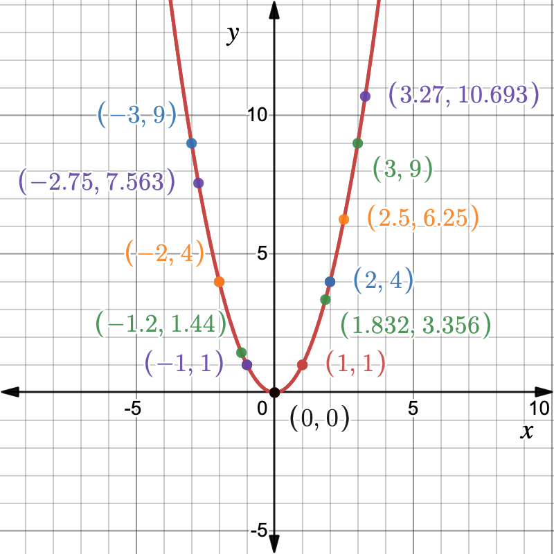
For example, starting with the table of values of \(f(x)=x^2\) in (b) of Figure 1.1.26 and adding a few additional input/out pairs (e.g., \((2.5, f(2.5))=(2.5, 6.25)\)), we are able to produce a convincing graph of \(f\text{.}\)
With a solid understanding of the precise relation between a function \(f\) and its graph, you will be able to easily translate visual features of the graph into corresponding properties of the function. As a general rule of thumb, horizontal features of the graph of a function \(f\) tell us something about the inputs of \(f\text{,}\) and vertical features tell us about its outputs.
For example, to infer the domain of a function from its graph, we simply take note of all the \(x\)-values of points \(P=(x,y)\) on the graph. This can be done visually by mentally “projecting” the points of the graph onto the \(x\)-axis and seeing what subset is produced. Similarly, the range of the function corresponds to the set of all \(y\)-values of points appearing in the graph, and this can be visualized by “projecting” all of the points of the graph onto the \(y\)-axis. Looking at the graph of \(f(x)=x^2\) given in Figure 1.1.29, and imagining this graph as continuing in a similar manner indefinitely to the left and right, we see that projecting points onto the \(x\)-axis produces the entire \(x\)-axis, whereas projecting onto the \(y\)-axis yields only the nonnegative portion of the \(y\)-axis. This is visual confirmation that the domain of \(f\) is all of \(\R\text{,}\) whereas the range of \(f\) is just \([0,\infty)\text{.}\)
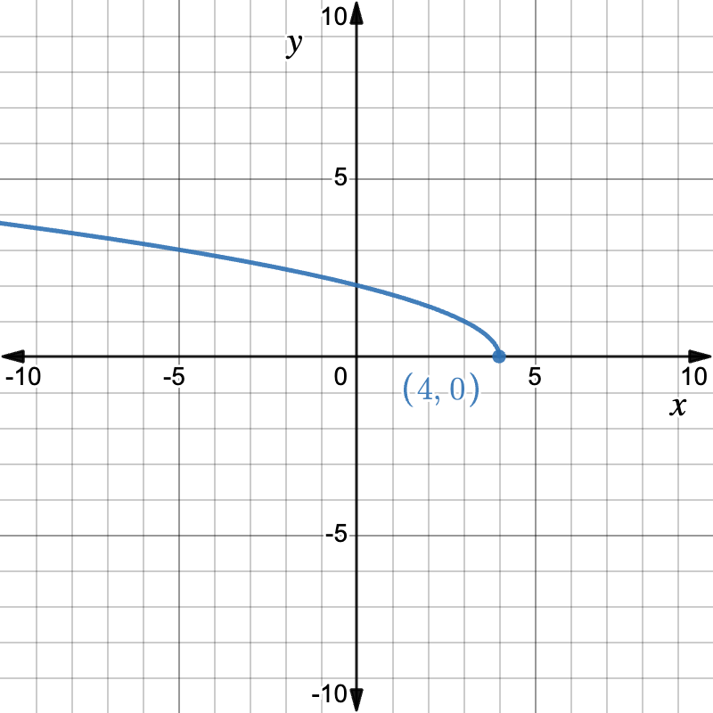
We see that the \(x\)-values of points on the graph of \(g\) seem to range over all real numbers less than or equal to \(4\text{.}\) This suggests that the domain of \(g\) is \((-\infty, 4]\text{.}\) To confirm this observe that the expression \(\sqrt{4-x}\) is defined only if \(4-x\geq 0\text{.}\) Now solve this inequality for \(x\text{:}\)
The \(y\)-values of the points of the graph of \(g\) appear to range over all of \([0,\infty)\text{.}\) We thus infer that the range of \(g\) is \([0,\infty)\text{.}\) (And indeed, this claim is readily confirmed using arguments as in Example 1.1.24 and Example 1.1.25.)
As we trace points on the interactive in Figure 1.1.33, we see that the \(x\)-values of points on the graph of \(h\) appear to assume all values with the exception of \(-2\) and \(2\text{,}\) suggesting that the domain of \(h\) is
We confirm this algebraically by first noting that the expression \(1/(x^2-4)\) is undefined exactly when \(x^2-4=0\text{.}\) Now solve this equation:
\begin{align*}
x^2-4 \amp =0\\
x^2 \amp =4 \\
x \amp =2 \text{ or } x=-2\text{.}
\end{align*}
(We review in more detail how to solve equations like \(x^2-4=0\) in Section 1.2.) We conlude that \(1/(x^2-4)\) is defined as long as \(x\ne \pm 2\) and thus that
Tracing points in the interactive, we observe that for points in the left- and right-most portions of the graph, the \(y\)-values of points assume all values except \(0\text{.}\) (As we move points to the left or right indefinitely, the graph gets very close to the \(x\)-axis, but never quite touches it.) On the other hand, for points in the middle section of the graph (between the lines \(x=-2\) and \(x=2\)), the \(y\)-values appear to range freely over the interval \((-\infty, -1/4]\text{.}\) We infer from these two observations that
where \(F(x,y)\) is a mathematical expression in the unknowns \(x\) and \(y\text{,}\) and \(c\in \R\) is a fixed constant. A solution to (1.9) is a pair \((a,b)\in \R^2\) such that evaluating the expression (1.9) at \(x=a\) and \(y=b\) yields the true equation
as an example. Let’s first try and produce a few solutions \((x,y)\) to this equation by hand. One trick that often comes in handy is to set one of the variables equal to zero and see what the other variable must be to produce a solution. Setting \(x=0\) in (1.10) reduces the equation to
\begin{equation*}
y^2=16\text{,}
\end{equation*}
which implies that \(y=\pm\sqrt{16}=\pm 4\text{.}\) We conclude that \((0,4)\) and \((0,-4)\) are solutions to (1.10). Similarly, setting \(y=0\) gives rise to the solutions \((4,0)\) and \((-4,0)\text{.}\) In all, we have managed to produce a set of four solutions to the equation:
This is far from the set of all solutions however. Indeed, observe that for each assignment \(x=t\) with \(t\in [-4,4]\) the expression \(16-t^2\) is nonnegative, and hence we can solve
\begin{equation*}
y^2=16-t^2
\end{equation*}
as \(y=\pm \sqrt{16-t^2}\text{.}\) This means for each \(t\in [-4,4]\text{,}\) the pairs
This yields infinitely many solutions to (1.10): two for each choice of \(t\in [-4,4]\text{.}\) For example, setting \(t=3\) in the expressions above yields the solutions \((3,\sqrt{5})\) and \((3,-\sqrt{5})\text{.}\)
We can use technology to produce a detailed graph of (1.10). Alternatively, you might recognize this equation as defining a certain circle centered at the origin. (Don’t worry if you didn’t catch this! We will review such special equations in much more detail later.) Below we provide this graph, along with the few points we managed to produce by hand.
The graph of equation (1.10) displayed in Figure 1.1.35 is similar in nature to the examples in the previous subsection. In particular, all of these graphs are curves of some sort in \(\R^2\text{.}\) One explanation of this similarity is that a graph of a function is just a specific example of a graph of an equation. Indeed, given function \(f\colon D\rightarrow \R\text{,}\) its graph
is just the graph of the equation \(f(x)=y\) (with the restriction that \(x\)-values of solutions must lie in \(D\)). So are there any differences between graphs of functions and graphs of curves more generally? Yes! The defining property of a function is that for each input \(x\in D\) of a function \(f\text{,}\) there is exactly one input/output pair \((x,f(x))\) on the graph of \(f\text{.}\) Graphically, this means that for each point \(t\) on the \(x\)-axis, there is at most one point on the graph of \(f\) with \(x\)-coordinate equal to \(t\text{:}\) equivalently, there is at most one point of the graph of \(f\) lying on the line \(x=t\text{.}\) This simple observation is the essence of the vertical line text.
The quantifiers “for all” and “there is” appearing in Theorem 1.1.36 are very important. To clarify their role in the statement of the theorem, let’s introduce some additional terminology. Given a vertical line \(L\text{,}\) let’s say that a set \(C\subseteq \R^2\) passes the \(L\)-test if \(L\) intersects \(C\) in at most one point; similarly, we will say \(C\) fails the \(L\)-test if \(L\) intersects \(C\) in more than one point. In terms of this new language, we see that the vertical line test asserts that \(C\) is the graph of a function if it passes the \(L\)-test for all vertical lines \(L\) in \(\R^2\text{;}\) and conversely, \(C\) is not the graph of a function if \(C\) fails the \(L\)-test for some vertical line \(L\) in \(\R^2\text{.}\)
Let’s see how this plays out with the graph \(C\) of equation (1.10). As illustrated in Figure 1.1.37, there are three qualitatively different ways in which a given vertical line \(L\) can intersect with \(C\text{.}\)
If the line \(L\) lies strictly to the left or right of \(C\text{,}\) then \(L\) does not intersect with \(C\) at all, and hence \(C\) passes the \(L\)-test.
If the line \(L\) is one of the two vertical lines \(x=-4\) or \(x=4\text{,}\) then \(L\) intersects \(C\) in exactly one point, and hence \(C\) passes the \(L\)-test.
Lastly, if \(L\) lies strictly between the lines \(x=-4\) and \(x=4\text{,}\) then \(L\) intersects \(C\) in exactly two points, and thus \(C\) fails the \(L\)-test.
Since \(C\) fails the \(L\)-test with respect to some vertical line (e.g., the line \(x=3\)), we conclude by Theorem 1.1.36 that \(C\) is not the graph of a function.
It might be helpful to envision the vertical line test as a scanning procedure. Imagine scanning your set \(C\subseteq \R^2\) with a device that produces a vertical green line \(L\) that we move from left to right across the entire expanse of \(C\text{.}\)
If at some moment while we are scanning from left to right our green vertical line \(L\) hits two or more different points on the graph, then our scanner emits a loud error beep, indicating that \(C\) has failed an \(L\)-test, and declares that \(C\) is not the graph of a function.
If, on the other hand, we are able to scan the entire expanse of \(C\) from left to right without hearing the error beep, then \(C\) has passed the \(L\)-test for all vertical lines \(L\text{,}\) and the scanner declares that \(C\) is the graph of a function.
Example1.1.39.Vertical line test: radical function.
Let \(f(x)=\sqrt{4-x}\) and let \(C\) be the graph of \(f\text{,}\) as depicted in Figure 1.1.31.
Suppose the line \(L\) has equation \(x=t\text{,}\) where \(t\in (-\infty, 4]\text{.}\) How many points lie in the intersection of \(L\) and \(C\text{.}\) Does \(C\) pass the \(L\)-test for this line \(L\text{?}\)
Suppose the line \(L\) has equation \(x=t\) with \(t\in (4,\infty)\text{.}\) How many points lie in the intersection of \(L\) and \(C\text{.}\) Does \(C\) pass the \(L\)-test in for this line \(L\text{?}\)
Graphically, for such lines \(L\text{,}\) we see that \(L\) intersects \(C\) in exactly one point. In more detail, if \(L\) has equation \(x=t\) with \(t\in (-\infty, 4]\text{,}\) then \(L\) intersects \(C\) at the point
If \(L\) has equation \(x=t\) with \(t\in (4,\infty)\text{,}\) then we see graphically that \(L\) does not intersect \(C\) at all, and hence \(C\) passes the \(L\)-test.
Since the lines discussed in (1) and (2) cover all possible lines in \(\R^2\text{,}\) and since we saw that \(C\) passes the \(L\)-test for all these lines \(L\text{,}\) we conclude by vertical line test that \(C\) is the graph of a function.
Students are sometimes perplexed that if a vertical line \(L\) does not intersect \(C\text{,}\) then \(C\) still passes the \(L\)-test. Example 1.1.39 is helpful in clearing up this confusion. There we see that the lines \(L\) with equation \(x=t\) that do not intersect \(C\) are precisely those for which \(t\notin (-\infty, 4]\text{,}\) the domain of \(f(x)=\sqrt{4-x}\text{.}\) The observation holds more generally: if \(C\) is the graph of a function \(f\colon D\rightarrow \R\text{,}\) then a line \(L\) with equation \(x=t\) intersects \(C\) in exactly one point if \(t\in D\) and does not intersect \(C\) at all for if \(t\notin D\text{.}\) This is because \(C\) only contains points of the form \((x,f(x))\text{,}\) where \(x\in D\text{.}\)
Yet another way of interpreting a function is as a binary relation (or just relation, for short). Loosely speaking, a binary relation \(R\) is a property that either holds (i.e., is true) or does not hold (i.e., is not true) for a given pair of elements \((x,y)\text{.}\) When the property holds for \((x,y)\) we write \(R(x,y)\text{.}\) A familiar example of a binary relation from mathematics is furnished by the “less than” relation: we define \(R(x,y)\) to mean the real number \(x\) is less than the real number \(y\text{,}\) denoted \(x< y\) in mathematical notation. For an example outside of mathematics, consider the binary relation \(R(x,y)\) defined as “\(x\) is a cousin of \(y\)”. In this case \(R(x,y)\) is true exactly when persons \(x\) and \(y\) are cousins.
A function \(f\colon A\rightarrow B\) gives rise to a binary relation \(R\) in a natural way: namely, we can define the relation \(R(x,y)\) as “\(y\) is the value of \(f\) at \(x\)” (or \(y=f(x)\text{,}\) for short). For example, the function \(f\colon \R\rightarrow \R\) defined as \(f(x)=x^2\) gives rise to the relation \(R(x,y)\) defined as \(y=x^2\text{,}\) or in plainer English, “\(y\) is the square of \(x\)”. For example, in this case \(R(2,4)\) is true, since \(4\) is the square of \(2\) (i.e., \(4=2^2\)), but \(R(4,2)\) is not true since \(2\) is not the square of \(4\) (i.e., \(2\ne 4^2\)).
Thus, we see that every function can be thought of as a certain binary relation. As with the situation with graphs of equations, however, not every relation arises from a function in this way. What makes relations arising from functions special is the defining property of a function: namely, that for every input \(x\) of a function \(f\text{,}\) there is exactly one output \(y=f(x)\text{.}\) As a consequence a relation \(R(x,y)\) is of the form \(y=f(x)\) for some function \(f\) if and only if for every \(x\) there is at most one \(y\) such that \(R(x,y)\) is true. This is just a logical analogue of the vertical line test!
We will say that a relation \(R(x,y)\) defines \(y\) as a function of \(x\) if there is a function \(f\) such that \(R(x,y)\) is true if and only if \(x\) is in the domain of \(f\) and \(y=f(x)\text{.}\) From our discussion above, it follows that a relation \(R(x,y)\) defines \(y\) as a function of \(x\) if and only if for every \(x\) there is at most one \(y\) such that \(R(x,y)\) is true.
Consider again the relation \(R(x,y)\) defined as “\(x\) is a cousin of \(y\)”. This relation does not define \(y\) as a function of \(x\) since it is possible for a person \(x\) to have more than one cousin.
Note that both \(R(4,2)\) and \(R(4,-2)\) are true, since \(2\) and \(-2\) are both square roots of \(4\text{.}\) Thus it is not the case that for all \(x\) there is at most one \(y\) such that \(R(x,y)\) is true. We conclude that this relation does not define \(y\) as a function of \(x\text{.}\)
In this case the relation \(R\) does define \(y\) as a function of \(x\text{.}\) This is because for each real number \(x\) there is at most one nonnegative square root. More explicitly, defining \(f(x)=\sqrt{x}\text{,}\) we see that \(R(x,y)\) is true if and only if \(y=f(x)\text{.}\)
The given relation \(R(x,y)\) does not define \(y\) as a function of \(x\) for the simple reason that a person \(x\) can have more than one phone number!
The answer here is perhaps somewhat debatable. If we agree that a given phone number can “belong” to at most one person, then \(R\) arises from the function \(f\) defined as follows: given a (registered) phone number \(x\text{,}\)\(f(x)\) is the owner of phone number \(x\text{.}\)
Why is this debatable? Well, for one thing, in the era before mobile phones, households were equipped with a single phone (called a “land line”), and the case could be made that that number was “owned” by all the people in the household. Thus, if we want to make a function out of this example, we would have to take more care to define what it means for a phone number to belong to a user.
This discussion is meant to be amusing, but is not entirely idle. It is often the case that a proposed function turns out upon closer inspection to not be well defined. Indeed, something very similar went wrong with the proposed function in Example 1.1.7.
Now that we have taken our first confident strides down the path of function exploration, you may be wondering why the study of functions is so important in the first place. The short answer is that functions are one of the most fundamental tools for modeling empirical phenomena. Scientific inquiry will often begin by treating one empirical quantity \(q\) as being determined or dependent on some other empirical quantity \(x\) (or even multiple quantities \(x_1, x_2,\dots, x_n\) in a multivariable model). In this situation it is natural to model the quantity \(q\) as a function of these other quantities: i.e., we assume there is a function \(f\) satisfying \(q=f(x)\) (or \(q=f(x_1,x_2,\dots, x_n)\) in a multivariable model). Here are some typical examples.
We can model the vertical velocity \(v\) of a skydiver in free fall as a function of the time \(t\) elapsed since the diver jumped from the plane. In this case we assume \(v=f(t)\) for some function \(f\text{.}\)
We can model the atmospheric temperature \(T\) as a function of altitude \(a\text{.}\) In this case we assume \(T=f(a)\) for some function \(f\text{.}\)
We can model the yearly sales \(S\) of a certain product as a function of its price \(p\) and the yearly amount \(a\) the producer spends on advertising. In this case we assume \(S=f(p,a)\) for some (multivariable) function \(f\text{.}\)
Observe how in these modeling situations the defining characteristic of a function \(f\text{,}\) that each input \(x\) has a unique output \(f(x)\text{,}\) captures our intuitive idea of one quantity being dependent on another. Indeed, this is what motivates the language of dependent and independent variables introduced in Remark 1.1.4. Checkpoint 1.1.42 leads you through a simplified simulation of how scientists proceed from observations of physical phenomena to a full-fledged mathematical model. You are encouraged to explore that exercise on your own.
In the meantime, we end this first section by giving a preview of what calculus is, and how it plays an important role in empirical modeling. In short, calculus is the science of functions. It provides us powerful tools to study properties of functions. What kind of properties of functions are we interested in determining? Continuing with the empirical modeling context, suppose we are modeling quantity \(q\) as a function \(q=f(s)\) of quantity \(s\) (i.e., quantity \(q\) is dependent on, or determined by quantity \(s\)). Here are some natural questions about \(f\) we are interested in when studying the function \(f\) that articulates the relation between \(s\) and \(q\text{.}\)
Maximum/minimum values.
Is there a maximum value of \(q\) that can be attained? Is there a minumum value? In terms of \(f\text{,}\) we are asking whether \(\range f\) has a maximum and/or minimum value. If it does, we would also like to know which inputs \(s\) give rise to these maximum and minimum values.
Perhaps \(q\) does not reach a maximum value. Does it approach some maximum value as \(s\) varies, without ever attaining that value? Suppose quantity \(s\) ranges naturally over the set \([0,\infty)\) of all nonnegative numbers: how does the output \(q=f(s)\) vary as \(s\) gets infinitely large?
How do the values \(q=f(s)\) change as we vary \(s\text{?}\) More specifically, does \(q\) increase as we increase \(s\text{?}\) Does \(q\) decrease as we increase \(s\text{?}\)
Fix a particular value \(s_0\) of our quantity \(q\text{,}\) and let \(q_0=f(s_0)\) be the value of \(q\) corresponding to that input. How does \(q_0\) change as we vary \(q\) by arbitrarily small amounts about \(q_0\text{.}\) More specifically, call
the average rate of change with respect to \(s\) as we vary \(s\) from \(s_0\) to \(s_1\text{.}\) What happens to these average rates of change if we keep \(q_0\) fixed, and pick \(q_1\) to be arbitrarily close to \(q\text{.}\) Do they approach a well-defined instantaneous rate of change?
All the questions above can be phrased as questions about the function \(f\) that models the relation between \(q\) and \(s\text{,}\) and we will be able to answer all of these questions, using calculus, by the end of this course!
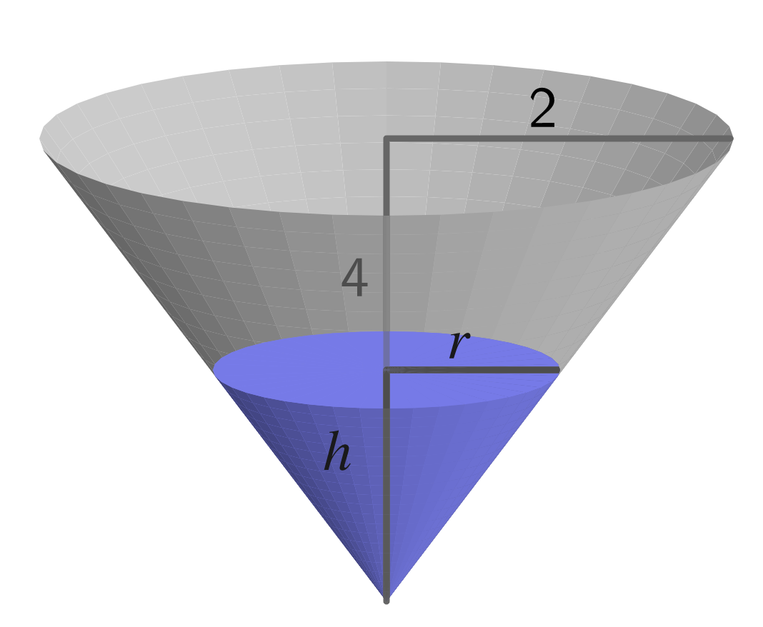
Figure 1.1.43 depicts a water tank in the shape of a circular cone (with tip pointed downward). The height of the tank is 4 meters, and its circular top has a radius of 2 meters. The tank contains an initial quantity of water that steadily drains through a regulated valve at the bottom.
Once the draining begins we record at each subsequent minute \(t\) the measurements of the height \(h\) (in meters), radius \(r\) (in meters), and volume \(V\) (in cubic meters) of the conical body of water remaining in the tank. These are summarized in Table 1.1.44.
It is evident that at any time \(t\) since the draining has begun, the height, radius, and volume of the remaining water have determinate values. Thus we have well-defined functions \(h=f_1(t)\text{,}\)\(r=f_2(t)\text{,}\) and \(V=f_3(t)\) that output the height, radius, and volume of the remaining water \(t\) minutes after draining has begun.
What is an appropriate domain \(D\) for the functions \(f_1,f_2,f_3\text{?}\) Our table only provides values of the functions for \(t\in \{0,1,2,3,4\}\text{.}\) Does this mean we should set \(D=\{0,1,2,3,4\}\text{?}\) (There is not one correct answer here.)
Focus on the measurements of the height \(h\) of the remaining water. How does the height change with each passing minute? Conjecture a formula for the function \(h=f_1(t)\text{.}\)
The table suggests a relation between the height \(h\) and radius \(r\) of the remaining water at any given time. Express this relation as an equation involving \(h\) and \(r\text{.}\) (This relation can in fact be proven using similar triangles, but you need not do this here.) Assuming your conjectured formula for \(f_1\) is correct, derive a formula for \(r=f_2(t)\text{.}\)
The volume formula for cylinders tells us that \(V=\frac{1}{3}\pi r^2\, h\text{.}\) Assuming your conjectured formula for \(f_1\) is correct, compute a formula for \(V=f_3(t)\text{.}\) Assess the accuracy of your formula by comparing its outputs with Table 1.1.44.
You have now modeled the various quanties associated to the remaining water with the functions \(f_1,f_2, f_3\text{.}\) Assess whether your model gives a sensible answer to the following question: what is the volume of the remaining water 10 minutes after the draining has begun? What, in the face of the evidence given by Table 1.1.44, is a plausible answer to this question. What is a natural way of adjusting your model so that it provides this answer?
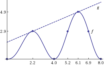
Based on the graphs of \(f(x)\) and \(g(x)\) below, answer the following questions. If a question has more than one answer, fill in your answer as a list of values separated by commas. Thus for example if you think \(f(x) = g(x)\) when \(x = 20\text{,}\) when \(x = 25\text{,}\) and when \(x = 29\text{,}\) you would enter 20, 25, 29 (or any other order of these three numbers separated by commas).
The table below \(A = f(d)\text{,}\) the amount of money \(A\) (in billions of dollars) in bills of denomination \(d\) circulating in US currency in 2005. For example according to the table values below there were $60.2 billion worth of $50 bills in circulation.
Chicago’s average monthly rainfall, \(R = f(t)\) inches, is given as a function of the month, \(t\text{,}\) where January is \(t = 1\text{,}\) in the table below.
A national park records data regarding the total fox population \(F\) over a 12 month period, where \(t = 0\) means January 1, \(t = 1\) means February 1, and so on. Below is the table of values they recorded:
(b) Let \(g(t) = F\) denote the fox population in month \(t\text{.}\) Find all solution(s) to the equation \(g(t) = 57\text{.}\) If there is more than one solution, give your answer as a comma separated list of numbers.
An open box is to be made from a flat piece of material 16 inches long and 2 inches wide by cutting equal squares of length \(x\)from the corners and folding up the sides.