Modeling with Linear and Quadratic Functions

Section 1.3 Modeling with Linear and Quadratic Functions

Subsection Learning Goals

Examine the mathematical modeling cycle.
🔗

🔗
Use linear and quadratic functions to describe real-world problems.
🔗

🔗
Practice translating back and forth between the context and mathematical calculations in a problem.
🔗

🔗
Revisit ideas of domain and range, increasing and decreasing, intercepts, and average rate of change in a context that gives these concepts a practical meaning.
🔗

🔗

Subsection The Mathematical Modeling Process

A mathematical model is a mathematical description (often by means of a function or an equation) of a real-world phenomenon such as the size of a population, the demand for a product, the speed of a falling object, the concentration of a product in a chemical reaction, the life expectancy of a person at birth, or the cost of emission reductions. The purpose of the model is to understand the phenomenon and perhaps to make predictions about future behavior.

🔗

Figure 1.3.1 below illustrates the process of mathematical modeling.

🔗

Figure 1.3.1. The modeling cycle. Graphic from www.educationaldesigner.org .
🔗

Given a real-world problem, our first task is to formulate a mathematical problem by

identifying and naming the independent and dependent variables
🔗

🔗
making assumptions that simplify the problem so it is easy enough to describe with mathematics
🔗

🔗
using knowledge of the physical situation to brainstorm relevant equations, formulas, and theorems, possibly working from data or a graph
🔗

🔗
obtaining equations that relate the variables
🔗

🔗

🔗

The second step is to apply the mathematics that we know (such as the calculus that we will be developing over the year) to the mathematical equations that we have formulated in order to derive a mathematical solution.

🔗

In the third step, we take those mathematical conclusions and interpret them as information about the original real-world phenomenon by way of offering explanations or making predictions. The final step is to test our predictions by checking against new real data. If the predictions don’t compare well with reality, we need to refine our model or formulate a new model and start the cycle over again.

🔗

This is similar to the framework for problem-solving described in Section 0.2, except that in a truly real-world problem, the actual question may not be stated explicitly or formulated in a way that can be answered without further refinement of the question (getting more information, simplifying more assumptions, building more theory). Since we are working in the context of a calculus course, all of our "real-world" questions will be very well-behaved and tractable.

🔗

A mathematical model is never a completely accurate representation of a physical situation. Instead, it is an idealization or an approximation. A good model simplifies reality enough to permit mathematical calculations but is accurate enough to provide valuable conclusions. It is important to realize the limitations of the model.

🔗

Subsection Average rate of change

In this section we will treat examples of modeling that use linear and quadratic functions. Important in this context is the question of why one of these types of functions would be more appropriate than the other in a given setting. One important difference between the two families of functions lies in the shape of their graphs: linear functions have linear graphs, whereas quadratic functions do not. (In fact the graph of a quadratic function is a parabola, as we will discuss later.)

🔗

The notion of the average rate of change of a function provides us with a convenient algebraic way of articulating this difference between linear and quadratic functions.

🔗

Definition 1.3.2. Average rate of change.

Assume the function $f$ is defined on the interval $[a,b]\text{.}$ The average rate of change from $a$ to $b$ (or over the interval $[a,b]$) is defined as

\begin{equation*} \frac{f(b)-f(a)}{b-a}\text{.} \end{equation*}

🔗

Remark 1.3.3. Average rate of change.

Some remarks are in order.

It is absolutely essential to note that the average rate of change of a function depends on the given interval. A function can possibly have one average rate of change on the interval $[0,1]$ and a different average rate of change on the interval $[1,2]\text{.}$
🔗

🔗
Let $y$ be the dependent variable for a function $f\text{,}$ so that $y=f(x)$ for all $x$ in the domain of $f\text{.}$ The average rate of change over an interval $[a,b]$ is a measure of how how quickly the the $y$-values of $f$ change as we let the input $x$ vary over $[a,b]\text{.}$ Writing $\Delta y=f(b)-f(a)$ and $\Delta x=b-a\text{,}$ to evoke change in $y$- and $x$-values respectively, we sometimes use the shorthand

\begin{equation*} \frac{f(b)-f(a)}{b-a}=\frac{\Delta y}{\Delta x}\text{.} \end{equation*}

This notation effectively evokes the concept of a rate of change. Note, however, that some important information is hidden in the $\Delta y/\Delta x$ notation, since the specific interval in question $[a,b]$ is not indicated in the notation.

🔗

🔗
In a modeling situation, the independent and dependent variables $x$ and $y$ usually have units attached to them. Using some “units algebra”, the units of the average rate of change over an interval $[a,b]$ are given as

\begin{equation*} \text{units of } \frac{f(b)-f(a)}{b-a}=\text{units of } \frac{\Delta y}{\Delta x}=\frac{\text{units } y}{\text{units } x}\text{,} \end{equation*}

usually read as “unit $y$ per unit $x$”. Making clear the units of an average rate of change often helps us understand the physical meaning of this measure in a modeling situation.

🔗

🔗
The average rate of change of a function $f$ over the interval $[a,b]$ is a somewhat coarse measure of how outputs of $f$ change with respect to inputs $x\in [a,b]$ as it only makes use of the information provided by the outputs $f(a)$ and $f(b)$ at the endpoints of this interval. This measure remains silent about what happens in between: i.e., it provides now information about how the function behaves on the open interval $(a,b)\text{.}$
🔗

🔗

🔗

The notion of average rate of change gives us an alternative characterization of a linear function: namely, a function $f\colon \R\rightarrow \R$ is linear if and only if its average rate of change is the same for any interval. We summarize this by saying that a linear function has a constant rate of change.

🔗

Theorem 1.3.4. Linear function equivalence.

Let $f\colon \R\rightarrow \R$ be a function. The following statements are equivalent.

$f$ is linear.
🔗

🔗
$f$ has a constant rate of change (i.e., the average rate of change of $f$ is the same for any interval).
🔗

🔗

Moreover, given a linear function $f(x)=mx+b\text{,}$ where $m$ and $b$ are constants, the slope $m$ is the average rate of change of $f$ over any interval $[c,d]\text{.}$ In other words, $m$ is the (constant) rate of change of $f\text{.}$

🔗

Proof.

Since we are proving the logical equivalence (1)$\iff$(2), we must show that (1)$\implies$(2) and (2)$\implies$(1). We show each implication separately.

🔗

Implication: (1)$\implies$(2).

Assume $f$ is linear. By definition this means there are constants $m,b\in \R$ such that $f(x)=mx+b$ for all $x\in \R\text{.}$ We claim that $m$ is the average rate of change of $f$ over any given interval. This means in particular that the average rate of change of $f$ is constant over any interval. To prove the claim we take any interval $I=[c,d]\text{,}$ and compute the average rate of change of $f$ over $I$ as

\begin{align*} \frac{f(d)-f(c)}{d-c} \amp =\frac{md+b-(mc+b)}{d-c} \amp (f(x)=mx+b) \\ \amp = \frac{md-mc}{d-c}\\ \amp = \frac{m(d-c)}{d-c}\\ \amp =m\text{,} \end{align*}

as desired.

🔗

Implication: (2)$\implies$(1).

Now assume that $f$ is a function whose average rate of change over any interval is always the same. Let $m$ be the value of this constant average rate of change. Furthermore, let $f(0)=b\text{.}$ We claim that $f(x)=mx+b$ for all $x\in \R\text{,}$ and hence that $f$ is linear. To prove the claim, let $x$ be any positive real number and consider the interval $I=[0,x]\text{.}$ Since the average rate of change of $f$ over $I$ is equal to the constant $m\text{,}$ we have

\begin{equation*} m=\frac{f(x)-f(0)}{x-0}=\frac{f(x)-b}{x}\text{.} \end{equation*}

Solving the equation above for $f(x)\text{,}$ we conclude that

\begin{equation*} f(x)=mx+b\text{.} \end{equation*}

Similarly, if $x$ is any negative real number, then applying the same argument to the interval $I=[x,0]\text{,}$ we conclude again that $f(x)=mx+b\text{.}$ Lastly, since $f(0)=b=m0+b\text{,}$ we see that $f(x)=mx+b$ for all $x\in \R\text{.}$ This proves $f$ is linear.

🔗

Example 1.3.5. Average rate of change: linear functions.

Decide from the given information whether the function $f$ is linear. If so, provide a formula for $f\text{.}$ (Assume the domain of $f$ is $\R\text{.}$)

Table 1.3.6. Table of values for $f$
🔗

x -3 -1 1 3

f(x) 10 7 4 1

🔗
Table 1.3.7. Table of values for $f$
🔗

x 2 3 5 7

f(x) -5 -4 -3 -2

🔗

🔗

Solution.

From the given information we see that the rate of change of $f$ is constant over any interval, and equal to

\begin{equation*} m=\frac{f(-1)-f(-3)}{-1-(-3)}=\frac{7-10}{2}=-\frac{3}{2}\text{.} \end{equation*}

From Theorem 1.3.4 we conclude that $f$ is linear and of the form

\begin{equation*} f(x)=-\frac{3}{2}x+b \end{equation*}

for some $b\in \R\text{.}$ To determine $b\text{,}$ we can evaluate $f$ at any of the provided inputs and then solve for $b\text{.}$ Using the input $x=1\text{,}$ for example, we have

\begin{align*} f(1)=4 \amp \implies -\frac{3}{2}\cdot 1+b=4\\ \amp \implies b-\frac{3}{2}=4\\ \amp \implies b=4+\frac{3}{2}=\frac{11}{2}\text{.} \end{align*}

We conclude that $f(x)=-\tfrac{3}{2}x+\tfrac{11}{2}\text{.}$ Note that although we were not asked to do so, we can easily check our answer by verifying that

\begin{align*} f(-3) \amp = 10 \amp f(-1)\amp=7 \amp f(1)\amp=4 \amp f(3)\amp =1\text{.} \end{align*}

🔗

🔗
The function is not linear! Be careful, there was a slight trick involved here in that the $x$-values included in the table are not incremented by a constant amount. That is pretty unconventional for a table, but not expressly prohibited. Computing the average rate of change of $f$ over the two intervals $[2,3]$ and $[3,5]$ we get

\begin{align*} \frac{f(3)-f(2)}{3-2} \amp = \frac{-4-(-5)}{1}=1\\ \frac{f(5)-f(3)}{5-3} \amp =\frac{-3-(-4)}{2}=\frac{1}{2}\text{.} \end{align*}

Since these average rates of change are not the same, we conclude that $f$ is not linear.

🔗

🔗

🔗

Subsection Using Linear Functions as Models

The new characterization of linear functions in Theorem 1.3.4 makes clear the role of linear functions in modeling: we should chose a linear function as our model, when the output quantity changes at a constant rate with respect to the input quantity.

🔗

Example 1.3.8. Dolbear’s law.

Dolbear’s law relates the chirping of crickets to temperature.

Aside

In the late 1800s, the physicist Amos Dolbear was listening to crickets chirp and noticed a pattern: how frequently the crickets chirped seemed to be connected to the outside temperature. If we let $T$ represent the temperature in degrees Fahrenheit and $N$ the number of chirps per minute, we can summarize Dolbear’s observations in the following table.

🔗

Table 1.3.9. Data for Dolbear’s observations

🔗

$N$ (chirps/min)	40	80	120	160
$T$ ($^\circ$F)	$50^\circ$	$60^\circ$	$70^\circ$	$80^\circ$

For a mathematical model, we often seek an algebraic formula that captures observed behavior accurately and can be used to predict behavior not yet observed. When we graph the data, we can see a pattern that tells us what kind of formula to use.

🔗

Figure 1.3.10. Graph of Dolbear’s data relating rate of chirps $N$ (chirps/min) and temperature $T$ ($^\circ$F).
🔗

The data appear to fit a line, suggesting that $T$ can be modeled as a linear function of $N\text{:}$ i.e., we have

\begin{equation*} T=f(N)=m\, N+b \end{equation*}

for some constants $m,b\in \R\text{.}$ According to Theorem 1.3.4, $m$ can be computed as the average rate of change of $f$ over any interval of our choosing. The points Using the points $(40,50)$ and $(80,60)$ on our graph allow us to compute the average rate of change of $f$ over $[40,80]$ as

\begin{equation*} \frac{60-50}{80-40} = \frac{10}{40} = \frac{1}{4}\text{.} \end{equation*}

Thus we have $T=f(N)=\tfrac{1}{4}N+b\text{.}$ Now evaluate this equation with any input/output pair you like in order to solve for $b\text{.}$ Taking $(N,P)=(40,50)\text{,}$ for example we see that:

\begin{align*} 50=f(40) \amp \implies 50=\frac{1}{4}\cdot 40+b\\ \amp \implies 50=10+b\\ \amp \implies b=50\text{.} \end{align*}

🔗

Before we attempt any further calculations, we may want to check that our model accurately represents the collected data. Let’s check that the point $(120,70)$ is indeed on the line. For $N=120\text{,}$ we have

\begin{equation*} T=0.25(120)+40 = 30+40 = 70 \end{equation*}

🔗

Success! We conclude that Dolbear’s function

\begin{equation} T=f(N)=\frac{1}{4}\, N+40\tag{1.28} \end{equation}

models the relationship between the number $N$ of cricket chirps per minute and the temperature $T$ in degrees Fahrenheit.

🔗

Checkpoint 1.3.11.

Now that we have a model for Dolbear’s observations, let’s use it to make some predictions.

If we hear snowy tree crickets chirping at a rate of 92 chirps per minute, what does Dolbear’s model suggest should be the outside temperature?
🔗

🔗
If the outside temperature is $77^\circ$ F, how many chirps per minute should we expect to hear?
🔗

🔗
Suppose that in the morning an observer hears 65 chirps per minute, and several hours later hears 75 chirps per minute. How much has the temperature risen between observations?
🔗

🔗

🔗

Example 1.3.12. Dolbear’s law: continued.

Let’s continue to explore the limits of our model for Dolber’s observations. Suppose we wish to know the number of chirps we should hear when the outside temperature is $35^\circ$ F. There is no point on the graph with $T=35$ and so we solve numerically for $N$ to determine the number of chirps one should hear when the outside temperature is $35^\circ$ F.

\begin{equation*} \begin{aligned}35\amp =40+0.25N\\ -5 \amp = 0.25N\\ -20 \amp =N \end{aligned} \end{equation*}

🔗

In context, this means that when it’s $35^\circ$ outside, we should hear $-20$ chirps per minute. A negative number of chirps per minute does not make sense, and so we can see that the model is not valid when the outside temperature is $35^\circ$ F.

🔗

At this point in the modeling process, a scientist would need to revisit the physical situation and make further observations. Indeed, Dolbear observed that temperatures below $50^\circ$ F are too cold for the crickets and temperatures above $85^\circ$ F are too hot for the crickets, so the model is only accurate for temperatures between $50^\circ$ F and $85^\circ$ F. Recalling that here we are modeling temperature $T$ as a function $T=f(N)$ of the rate of chirping $N\text{,}$ we see that for our model to be meaningful, we want $\range f$ (set of outputs $T$) to lie in $[50,85]\text{.}$ Since our function $f$ is linear, this means we must restrict the domain (possible $N$ inputs) accordingly. First let’s solve the equations $50=f(N)$ and $85=f(N)$ for $N\text{:}$

\begin{align*} 50=f(N) \amp \implies 50=\frac{1}{4}\, N+40\\ \amp \implies N=40 \\ 80=f(N) \amp \implies 85=\frac{1}{4}\, N+40\\ \amp \implies N=180\text{.} \end{align*}

Since $f$ is an increasing function of $N\text{,}$ it follows that if we want $\range f=[50, 85]\text{,}$ we need to pick the domain of $f$ to be $D=[40, 180]\text{.}$

🔗

Remark 1.3.13. Domains of modeling functions.

When working with a model, it is common to have to restrict the domain of a function based on real-world conditions, rather than algebraic requirements, so that the model makes sense in the context it is meant to represent.

🔗

Here is another physical phenomenon where a linear function provides an appropriate model: measuring the area of a glacier over time. Remember: linear functions have constant average rates of change, so are ideal for modeling quantities that change at a constant rate.

🔗

Example 1.3.14. Modeling Glacier Areas.

The summit of Africa’s largest peak, Mt. Kilimanjaro, has two main ice fields and a glacier at its peak. Geologists measured the ice cover in the year 2000 ($t=0$) to be approximately $1951$ m$^2\text{;}$ in the year 2007, the ice cover measured $1555$ m$^2\text{.}$

Suppose that the amount of ice cover at the peak of Mt. Kilimanjaro is changing at a constant average rate from year to year. Find a linear model $A=f(t)$ whose output is the area, $A$ in square meters in year $t$ (where $t$ is the number of years after 2000).
🔗

🔗
What do the slope and $A$-intercept mean in the model you found in (a)? In particular, what are the units on the slope?
🔗

🔗
Compute $f(17)\text{.}$ What does this quantity measure? Write a complete sentence to explain.
🔗

🔗
If the model holds further into the future, when do we predict the ice cover will vanish?
🔗

🔗
In light of your work above, what is a reasonable domain to use for the model $A=f(t)\text{?}$ What is the corresponding range?
🔗

🔗

🔗

Solution.

We are told that the ice cover starts at $b=1951\text{,}$ so the point $(0,1951)$ lies on the graph of the function. We are also given the point $(7,1555)\text{.}$ The slope is then

\begin{equation*} \begin{aligned}m \amp = \frac{1555-1951}{7-0}\\ \amp = \frac{-396}{7}\\ \amp \approx -56.5714 \end{aligned} \end{equation*}

The linear model is then $A=f(t) = 1951-\frac{396}{7}t\text{.}$

🔗

🔗
The slope is the rate at which the glacier is losing ice each year, measured in m$^2$/year. The $A$-intercept is the area of the ice at $t=0$ (in 2000).
🔗

🔗
$f(17) = 1951-\frac{396}{7}(17)\approx 989.2857\text{.}$ In 2017, the ice cover on the glacier is approximately 989.2857 m$^2\text{.}$
🔗

🔗
The ice cover will vanish when $A=1951-\frac{396}{7}t=0\text{.}$ Solving for $t\text{,}$ we have $t\approx 34.4874\text{.}$ The ice cover will vanish toward the end of May of 2034.
🔗

🔗
A reasonable domain for the model is $t\in[0,34.4874]\text{.}$ The corresponding range is $A\in[0,1951]\text{,}$ meaning the ice cover will take on values between 1951 m$^2$ and 0 m$^2\text{.}$ (Note that we still write this interval as 0 to 1951 when using interval notation, even though the ice cover is vanishing.)
🔗

🔗

🔗

Checkpoint 1.3.15.

What is a quantity or phenomenon that you observe to have a constant rate of change? Assign names to the independent and dependent variables and create a linear model of this phenomenon. If relevant, include an appropriate domain and/or range. Is your model an increasing or decreasing linear function?

🔗

Subsection Modeling with quadratic functions: falling objects

One of the reasons that quadratic functions are so important is because of a physical fact of the universe we inhabit: for an object only being influenced by gravity, acceleration due to gravity is constant. If we measure time in seconds and a rising or falling object’s height in feet, the gravitational constant is $-32$ feet per second per second, where the negative sign signifies that gravity is pulling "down," meaning toward the ground.

🔗

One of the fantastic consequences of calculus — which, like the realization that acceleration due to gravity is constant, is largely due to Sir Isaac Newton in the late 1600s — is that the height of a falling object at time $t$ is modeled by a quadratic function.

🔗

Theorem 1.3.16. Height of falling object.

For an object tossed vertically from an initial height of $s_0$ feet with a velocity of $v_0$ feet per second, the object’s height at time $t$ (in seconds) is given by the formula

\begin{equation*} h(t) = -16t^2+v_0t+s_0 \end{equation*}

and corresponds to a gravitational constant of $g=-32$ ft/s$^2\text{.}$

🔗

If height is measured instead in meters and velocity in meters per second, the gravitational constant is $g=-9.8$ m/s$^2$ and the function $h$ has form $h(t) = -4.9t^2+v_0t+s_0\text{.}$

🔗

We will see where this formula comes from later in the course!

🔗

Example 1.3.17. Water ballon.

A water balloon is tossed vertically from a dorm room window at an initial height of 37 feet with an initial velocity of 41 feet per second.

Find a formula for the height $h(t)$ of the ballon $t$ seconds after it is tossed.
🔗

🔗
When does the balloon hit the ground?
🔗

🔗
Use technology to produce a graph of $h\text{,}$ and use this to estimate the maximum height reached by the water balloon during its flight.
🔗

🔗

🔗

Solution.

We can use Theorem Theorem 1.3.16 to model the height of the water balloon. First, we notice that since the information is given in feet and seconds, we should use the formula

\begin{equation*} h(t) = -16t^2+v_0t+s_0 \end{equation*}

corresponding to a gravitational constant of $-32$ ft/s$^2\text{.}$ Next, we determine the constants in the formula. The initial height in the problem is given as 37 feet, so we have

\begin{equation*} s_0 = 37\text{.} \end{equation*}

🔗

The initial velocity is given as 41 feet per second. Note the units! This is the rate of change of position. Thus we have

\begin{equation*} v_0 = 41\text{.} \end{equation*}

🔗

Thus our model is

\begin{equation*} h(t) = -16t^2+41t+37 \end{equation*}

where $t$ is measured in seconds, $t=0$ denotes the time at which the water balloon is thrown, and $h(t)$ is measured in feet.

🔗

🔗
The balloon hitting corresponds to a time $t$ when $h(t)=0\text{.}$ Thus, we wish to solve

\begin{equation*} h(t) = -16t^2+41t+37 = 0 \end{equation*}

for $t\text{,}$ noting that we would like to have a positive time since our model only becomes valid after $t=0\text{.}$ That quadratic equation does not look like it will factor nicely, so we will immediately use the quadratic formula:

\begin{equation*} \begin{aligned}t\amp = \frac{-b\pm\sqrt{b^2-4ac}}{2a}\\ \amp = \frac{-41\pm\sqrt{(41)^2-4(-16)(37)}}{2(-16)}\\ \amp = \frac{-41\pm\sqrt{4049}}{-32}\\ \amp \approx 3.2697, -0.7072 \end{aligned} \end{equation*}

🔗

Since we are looking for a time after the balloon is thrown, the answer we are looking for is

\begin{equation*} \text{ the balloon hits the ground approximately 3.27 seconds after it is thrown}\text{.} \end{equation*}

This implies a domain for our model since the balloon cannot pass through the ground: the model $h(t) = -16t^2+41t+37$ gives the height of the water balloon $t$ seconds after it is thrown until it hits the ground, so for $t\in[0,3.27]\text{.}$

🔗

🔗
Lastly, let’s graph our function and use that to estimate the time the water balloon reaches its highest point, along with its height at that time. This will give us the range of our model, as well.
🔗

Figure 1.3.18. The function $h=f(t)= -16t^2+41t+37$ that models the height of the water balloon for $t\in[0,3.27]\text{.}$
🔗
From the Desmos graph, we can see that the quadratic function reaches its maximum at approximately the point $(1.281, 63.266)\text{,}$ and that the range of our modeling function is $\range f=[0,63.266]\text{.}$ Interpreting this information back into the context of the balloon, we can say that the balloon reaches its highest point approximately $1.281$ second after it is thrown, and that its height is $63.266$ feet at that time.
🔗

Note that we can verify these claims algebraically by computing a completed square form of our quadratic function. We have

\begin{align*} h=f(t) \amp = -16t^2+41t+37\\ \amp =-16(t^2-41/16t)+37\\ \amp =-16(t-41/32)^2+(37+41^2/64)\text{.} \end{align*}

From Theorem 1.2.33, we conclude that $f$ has a maximum at

\begin{equation*} t=41/32\approx 1.281 \end{equation*}

and its maximum value there is

\begin{equation*} f(41/32)=(37+41^2/64)\approx 63.266\text{.} \end{equation*}

🔗

🔗

🔗

Checkpoint 1.3.19.

Use the model developed in Example Example 1.3.17 to answer the following questions.

Compute the average rate of change of $h$ on the interval $[1,2]\text{.}$ What are the units for the number you computed?
🔗

🔗
Copy the graph of $h(t)$ from Figure 1.3.18 to your notes. Draw an appropriate line on the graph whose slope is the value of the average rate of change in part (a).
🔗

🔗
You should have computed in part (a) and be able to see in part (b) that the average rate of change of $h$ on the interval $[1,2]$ is negative. Does this mean that the balloon is falling between $t=1$ and $t=2\text{?}$
🔗

🔗
Compute the average rate of change of $h$ on the interval $[2,3]\text{.}$ Is the balloon speeding up or slowing down as it approaches the ground?
🔗

🔗

🔗

Subsection Cost, Revenue, and Profit

In the business world the quantities of cost, revenue, and profit related to production of a good are of great importance. These quantities are often modeled as functions of the amount $q$ of the good produced.

🔗

Definition 1.3.20. Cost function.

The cost function $C=C(q)$ gives the total cost $C$ of producing a quantity $q$ of some good.

🔗

What sort of function do you expect $C=f(q)$ to be? The more goods that are made, the higher the total cost, so $C$ is an increasing function. Costs of production can be separated into two parts: the fixed costs, which are incurred even if nothing is produced, and the variable costs, which depend on how many units are produced.

🔗

Example 1.3.21. Radio production: cost function.

Let’s consider a company that makes radios. The factory and machinery needed to begin production are fixed costs, which are incurred even if no radios are made. The costs of labor and raw materials are variable costs since these quantities depend on how many radios are made. The fixed costs for this company are $24,000 and the variable costs are $7 per radio. Then

\begin{equation*} \begin{aligned}\text{ Total costs for the company } \amp = \text{ Fixed costs } +\text{ Variable costs } \\ \amp = 24,000 + 7\cdot\text{ Number of radios, } \end{aligned} \end{equation*}

so, if $q$ is the number of radios produced,

\begin{equation*} C= 24,000+7q\text{.} \end{equation*}

🔗

The variable cost for one additional unit is called the marginal cost. For a linear cost function, the marginal cost is the rate of change, or slope, of the cost function.

🔗

Checkpoint 1.3.22.

In each case, draw a graph of a linear cost function satisfying the given conditions:

Fixed costs are large but marginal cost is small.
🔗

🔗
There are no fixed costs but marginal cost is high.
🔗

🔗

🔗

Definition 1.3.23. Revenue Function.

The revenue function, $R=R(q)\text{,}$ gives the total revenue $R$ resulting from the production of a quantity $q$ of some good.

🔗

Let’s assume that the price of our good $p=p(q)$ is itself a function of the quantity $q$ of the good produced. Assuming further that the quantity of goods sold is equal to the quantity produced (not always a good assumption!), we conclude that revenue function $R(q)$ is computed as

\begin{equation} R(q) = \underset{p(q)}{\underbrace{\text{price}}}\cdot \underset{q}{\underbrace{\text{quantity}}}\text{.}\tag{1.29} \end{equation}

In the simplest case, the price $p$ is a constant, independent of the quantity of goods produced, in which case formula (1.29) reduces to $R(q)=pq\text{,}$ modeling revenue as a linear function of $q\text{.}$ In this case, the graph of $R(q)$ is a line passing through the origin with slope $p\text{.}$

🔗

Example 1.3.24. Radio production: revenue.

If radios sell for $15 each, then the manufacturer’s revenue function is

\begin{equation*} R(q) = pq = 15q \end{equation*}

🔗

Example 1.3.25. Radio production: cost and revenue.

Graph the cost function $C(q) = 24,000+7q$ and the revenue function $R(q) = 15q$ on the same axes. For what values of $q$ does the company make money?

🔗

Solution.

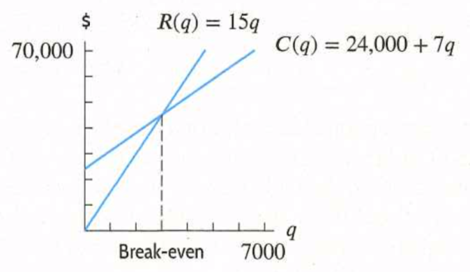
The company makes money whenever revenues are greater than costs, so we find the values of $q$ for which the graph of $R(q)$ lies above the graph of $C(q)\text{:}$

🔗

We find the point at which the graph of $R(q)$ and $C(q)$ cross:

\begin{equation*} \begin{aligned}\text{ Revenue } \amp = \text{ Cost } \\ 15q \amp = 24,000+7q\\ 8q \amp = 24,000\\ q \amp = 3000. \end{aligned} \end{equation*}

🔗

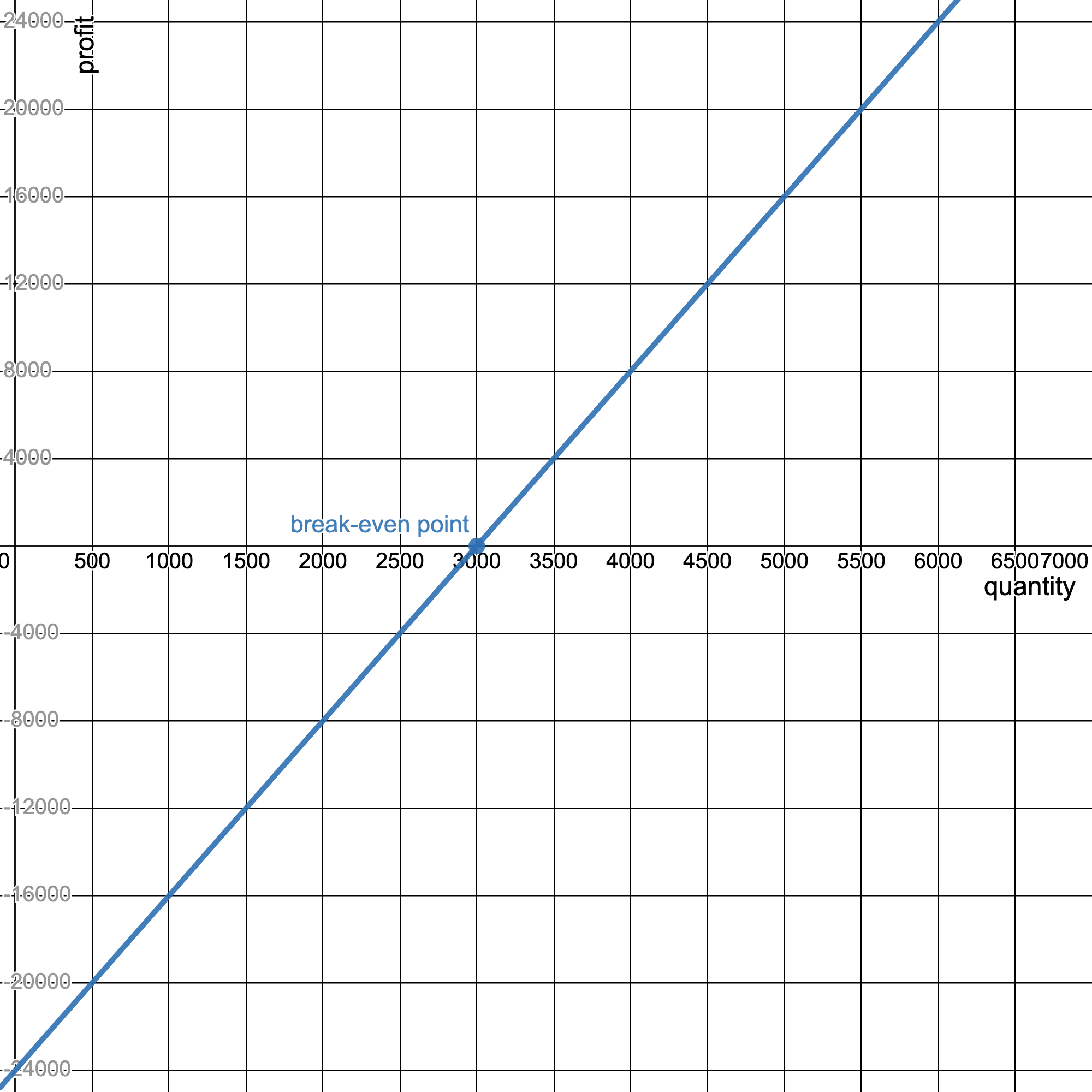
The company makes a profit if it produces and sells more than 3000 radios. The company loses money if it produces and sells fewer than 3000 radios.

🔗

This difference between the revenue and cost is called profit, and many decisions are made based on this quantity, rather than cost or revenue alone:

🔗

Definition 1.3.26. Profit function.

Assume the production of a certain good has associated cost and revenue functions $C(q)$ and $R(q)\text{,}$ where $q$ is the quantity of good produced. The profit function, denoted $\pi(q)$ is defined as

\begin{equation} \pi(q)=R(q)-C(q)\text{.}\tag{1.30} \end{equation}

In other words, $\pi(q)$ is the net profit (revenue minus cost) resulting from producing a quantity $q$ of the good.

🔗

The break-even point is the level of production $q$ resulting in a profit of zero: equivalently, this is the level of production where revenue equals cost.

🔗

Example 1.3.27. Radio production: break-even point and fixed cost.

For our radio manufacturer, a formula for the profit function is

\begin{equation*} \begin{aligned}\pi(q) \amp = R(q) - C(q)\\ \amp = 15q-(24,000+7q)\\ \amp =-24,000+8q \end{aligned} \end{equation*}

🔗

Notice that in terms of the graph of $\pi(q)\text{,}$ the fixed cost corresponds to the $y$-intercept, and the break-even point corresponds to the $x$-intercept.

🔗

Figure 1.3.28. Profit $\pi(q) = -24,000+8q$ for the radio manufacturer.
🔗

🔗

Checkpoint 1.3.29.

If cost, $C\text{,}$ and revenue, $R\text{,}$ are given by the graph below, what is the break-even point for the company? For what production quantities does the firm make a profit?

🔗

Just as we used the term marginal cost to mean the rate of change, or slope, of a linear cost function, we use the terms marginal revenue and marginal profit to mean the rate of change, or slope, of linear revenue and profit functions, respectively. The term marginal is used because we are looking at how the cost, revenue, or profit change "at the margin," that is, by the addition of one more unit.

🔗

Example 1.3.30.

For example, for the radio manufacturer, the marginal cost is 7 dollars/item (the additional cost of producing one more item is $7), the marginal revenue is 15 dollars/item (the additional revenue from selling one more item is $15), and the marginal profit is 8 dollars/item (the additional profit from selling one more item is $8).

🔗

Checkpoint 1.3.31.

How is the idea of a "marginal" cost, revenue, or profit similar to the idea of the average rate of change of a function?

🔗

Exercises Exercises

1.

A town has a population of $1400$ people at time $t=0\text{.}$ In each of the following cases, write a formula for the population $P\text{,}$ of the town as a function of year $t\text{.}$

🔗

(a) The population increases by $80$ people per year.

🔗

$P=$ people

🔗

(b) The population increases by $2$ percent a year.

🔗

$P=$ people

🔗

Answer 1.

$1400+80t$

🔗

Answer 2.

$1400\cdot 1.02^{t}$

🔗

Solution.

(a)$1400$$80\text{,}$$P=1400 +80 t\text{.}$(b)$1400$$2$$P=1400 (1.02)^t\text{.}$

🔗

2.

Let $t$ be time in seconds and let $r(t)$ be the rate, in gallons per second, that water enters a reservoir:

\begin{equation*} r(t)=600 - 35 t. \end{equation*}

🔗

(a) Evaluate the expression $\ r(10) =$

🔗

(b) Which one of the statements below best describes the physical meaning of the value of $r(10)$ ?

The rate, in gallons per second, at which the water is entering reservoir after 10 seconds.
🔗

🔗
The total amount, in gallons, of water in the reservoir after 10 seconds.
🔗

🔗
How many seconds until the water is entering to reservoir at a rate of 10 gallons per second.
🔗

🔗
The rate at which the rate of the water entering the reservoir is decreasing when 10 gallons remain in the reservoir.
🔗

🔗
None of the above
🔗

🔗

🔗

(c) For each of the mathematical expressions below, match one of the statements A - E below which best explains its meaning in practical terms.

🔗

The slope of the graph of $r(t)\text{.}$
🔗

🔗
The vertical intercept of the graph of $r(t)\text{.}$
🔗

🔗

The rate at which the rate of water entering the reservoir is decreasing in gallons per second squared.
🔗

🔗
After how many seconds the water stops flowing into the reservoir and starts to drain out.
🔗

🔗
The rate, in gallons per second, at which the water is initially entering the reservoir.
🔗

🔗
The initial amount of water, in gallons, in the reservoir.
🔗

🔗
The average rate, in gallons per second, at which water is flowing out of the reservoir.
🔗

🔗

🔗

(d) For $0 \leq t \leq 25\text{,}$ when does the reservoir have the most water?

🔗

When $t =$ sec.

🔗

(e) For $0 \leq t \leq 25\text{,}$ when does the reservoir have the least water?

🔗

When $t =$ sec.

🔗

(f) If the domain of $r(t)$ is $0 \leq t \leq 25\text{,}$ what is the range of $r(t)\text{?}$

🔗

range = (enter your answer in interval notation, or an inequality in $r\text{:}$ )

🔗

Answer 1.

$250$

Answer 2.

Answer 3.

Answer 4.

Solution.

SOLUTION$r(10) = 600 - 35(10)=250\text{.}$$r(10) = 250$$t = 10$$t = 0$$600/35 \approx 17.143$$-35\text{.}$$r(t)\text{,}$$t = 600/35$$t = 600/35\text{,}$$t= 600/35$$t= 25\text{,}$$t=0$$t=600/35\text{.}$$t=0\text{.}$$r(t)$$0 \leq t \leq 25$$t=0$$t=25\text{,}$$-275 \leq r(t) \leq 600\text{.}$$\lbrack -275, 600 \rbrack$

🔗

3.

A report by the US Geological Survey indicates that glaciers in Glacier National Park, Montana, are shrinking. Recent estimates indicate the area covered by glaciers has decreased from over $25.5 \ \mbox{km}^2$ in 1850 to about $16.5 \ \mbox{km}^2$ in 1995. Let $A = f(t)$ give the area (in square km) $t$ years after 2000, and assume $f(t) = 16.2 - 0.062t\text{.}$

🔗

a) Find and explain the meaning of the slope. Which statement best explains its significance?

The total area covered by glaciers decreased by $16.2 \ \mbox{km}^2$ from 1850 to 2000.
🔗

🔗
The area covered by glaciers is decreasing by $62,000 \ \mbox{m}^2$ every year.
🔗

🔗
The area covered by glaciers is decreasing by $62 \ \mbox{m}^2$ every year.
🔗

🔗
The area covered by glaciers is decreasing by $16.2 \ \mbox{km}^2$ every year.
🔗

🔗
The total area covered by glaciers is increasing by $0.062 \ \mbox{km}^2$ every year.
🔗

🔗
None of the above
🔗

🔗

🔗

b) Find and explain the meaning of the $A$-intercept. Which statement best explains its significance?

The area covered by glaciers is decreasing by $16.2 \ \mbox{km}^2$ every year.
🔗

🔗
The area covered by glaciers in 2000 was $16.2 \ \mbox{km}^2\text{.}$
🔗

🔗
The total area covered by glaciers decreased by $16.2 \ \mbox{km}^2$ from 1850 to 2000.
🔗

🔗
The area covered by glaciers in 2000 was $0.062 \ \mbox{km}^2$ .
🔗

🔗
The total area covered by glaciers will decrease by $0.062 \ \mbox{km}^2$ from 2000 to 2001.
🔗

🔗
None of the above
🔗

🔗

🔗

c) For both expressions listed below, enter the letter A-E of the statement which best explains their practical meaning. There are extra, unused statements.

$f( 12 )$ is
🔗

🔗
If $f(t) = 12\text{,}$ then $t$ is
🔗

🔗

The number of years after 2000 that the amount of glacier area that has disappeared is $12 \ \mbox{km}^2\text{.}$
🔗

🔗
The amount of glacier area (in $\mbox{km}^2$) that disappears in 12 years.
🔗

🔗
How much area (in $\mbox{km}^2$) will be covered by glaciers in 2012.
🔗

🔗
How much area (in $\mbox{km}^2$) will be covered by glaciers in 12 years.
🔗

🔗
The number of years after 2000 that the total area covered by glaciers will be $12 \ \mbox{km}^2\text{.}$
🔗

🔗

🔗

d) Evaluate $f( 12 ) =$

🔗

e) How much glacier area disappears in 12 years? $\mbox{km}^2$

🔗

f) Solve $f(t) = 12$ . $t =$ (round your answer to one decimal place)

Answer 1.

Answer 2.

Answer 3.

Solution.

SOLUTION$m = 0.062\text{,}$$0.062 \ \mbox{km}^2$$1 \ \mbox{km}^2 = 1,000,000 \ \mbox{m}^2\text{.}$$62,000 \ \mbox{m}^2$$A$$b = 16.2\text{,}$$16.2 \ \mbox{km}^2\text{.}$$f( 12 )$$f(t) = 12$$12 \ \mbox{km}^2\text{.}$$f( 12 ) = 16.2 - 0.062( 12) = 15.456$$m = \frac{ \Delta A }{ \Delta t } = -0.062\text{.}$$\Delta t = 12$$\frac{ \Delta A }{ 12 } = -0.062$$\Delta A = - 0.744\text{.}$$\mbox{km}^2$$16.2 - 0.062 t = 12\text{,}$$- 0.062 t = -4.2\text{,}$$t \approx 67.7\text{.}$

🔗

4.

If a ball is thrown straight up into the air with an initial velocity of $90$ ft/s, its height in feet after $t$ second is given by $y = {90}t - 16t^2\text{.}$ Find the average velocity (include units, ) for the time period begining when $t = 2$ seconds and lasting

(i) $0.5$ seconds

Average velocity:

(ii) $0.1$ seconds

Average velocity:

(iii) $0.01$ seconds

Average velocity:

Finally based on the above results, guess what the instantaneous velocity of the ball is when $t =2\text{.}$

🔗

Average velocity:

🔗

Answer 1.

$18\ {\textstyle\frac{\rm\mathstrut ft}{\rm\mathstrut s}}$

🔗

Answer 2.

$24.4\ {\textstyle\frac{\rm\mathstrut ft}{\rm\mathstrut s}}$

🔗

Answer 3.

$25.84\ {\textstyle\frac{\rm\mathstrut ft}{\rm\mathstrut s}}$

🔗

Answer 4.

$26\ {\textstyle\frac{\rm\mathstrut ft}{\rm\mathstrut s}}$

🔗

Prev Top Next

\(N\) (chirps/min)	40	80	120	160
\(T\) (\(^\circ\)F)	\(50^\circ\)	\(60^\circ\)	\(70^\circ\)	\(80^\circ\)

x	-3	-1	1	3
f(x)	10	7	4	1

x	2	3	5	7
f(x)	-5	-4	-3	-2

Section 1.3 Modeling with Linear and Quadratic Functions

Subsection Learning Goals

Subsection The Mathematical Modeling Process

Subsection Average rate of change

Definition 1.3.2. Average rate of change.

Remark 1.3.3. Average rate of change.

Theorem 1.3.4. Linear function equivalence.

Proof.

Implication: (1)\(\implies\)(2).

Implication: (2)\(\implies\)(1).

Example 1.3.5. Average rate of change: linear functions.

Subsection Using Linear Functions as Models

Example 1.3.8. Dolbear’s law.

Aside

Checkpoint 1.3.11.

Example 1.3.12. Dolbear’s law: continued.

Remark 1.3.13. Domains of modeling functions.

Example 1.3.14. Modeling Glacier Areas.

Checkpoint 1.3.15.

Subsection Modeling with quadratic functions: falling objects

Theorem 1.3.16. Height of falling object.

Example 1.3.17. Water ballon.

Checkpoint 1.3.19.

Subsection Cost, Revenue, and Profit

Definition 1.3.20. Cost function.

Example 1.3.21. Radio production: cost function.

Checkpoint 1.3.22.

Definition 1.3.23. Revenue Function.

Example 1.3.24. Radio production: revenue.

Example 1.3.25. Radio production: cost and revenue.

Definition 1.3.26. Profit function.

Example 1.3.27. Radio production: break-even point and fixed cost.

Checkpoint 1.3.29.

Example 1.3.30.

Checkpoint 1.3.31.

Exercises Exercises

1.

2.

3.

4.