Having become more or less acquainted with a few families of functions (linear functions, power functions, polynomials, rational functions, etc.), we now try to extend our knowledge to various arithmetic combinations of these basic types.
In this section we will focus on a particularly simple case of such combinations. Namely, we will consider the following types of function operations, called function transformations:
where \(c\) is a constant. In each case above, the function \(g\) above is the result of a “shifting” or “scaling” by the constant \(c\text{;}\) and furthermore, this shifting/scaling is applied either to the output\(f(x)\) (the “outside” of the function), or to the input\(x\) (the “inside” of the function). What exactly is the result of this shifting and scaling, and what difference does it make to do so on the inside versus the outside of the function?
The Desmos interactive in Figure 1.6.2 allows you to explore the graphical relationship between an original function \(f\) and four different type of transformations of \(f\text{:}\)
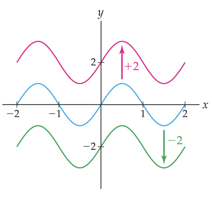
Hopefully, the Desmos interactive strongly suggests a graphical interpretation of each of the four different types of transformations. Our next two examples take on the two additive transformations:
is the observation that a point \(P=(x,y)\) lies on the graph of \(f\) if and only if the point \(Q=(x,y+c)\) lies on the graph of \(g\text{.}\) This is because
As a result, the graph of \(g(x)=f(x)+c\) is obtained from the graph of \(f\) by “shifting” it a directed distance of \(c\) units. The modifier “directed” is used here to take notice of the sign of \(c\text{.}\) More directly, assuming \(c\geq 0\text{,}\) we have the following graphical interpretation:
the graph of \(g(x)=f(x)+c\) is obtained from the graph of \(f\) by shifting up\(c\) units;
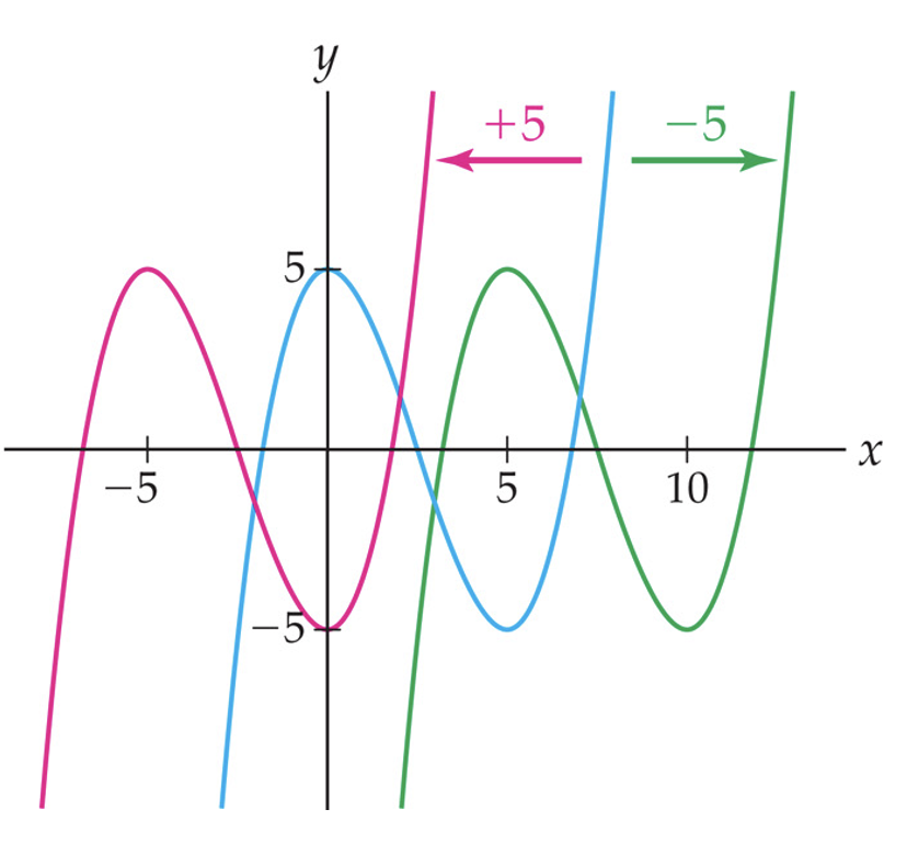
we observe that a point \(P=(x,y)\) lies on the graph of \(f\) if and only if the point \(Q=(x-c, y)\) lies on the graph of \(g\text{.}\) This is because
As a result, we obtain the graph of \(g(x)=f(x+c)\) by “shifting” the graph of \(f\) by the directed distance \(-c\text{.}\) More directly, assuming \(c\geq 0\text{,}\) we conclude:
the graph of \(g(x)=f(x+c)\) is obtained from the graph of \(f\) by shifting \(c\) units to the left;
For these transformations, both the sign and size of the constant \(c\) have a significant effect on the resulting graphical transformation. Our next examples consider the case where \(c> 0\text{.}\)
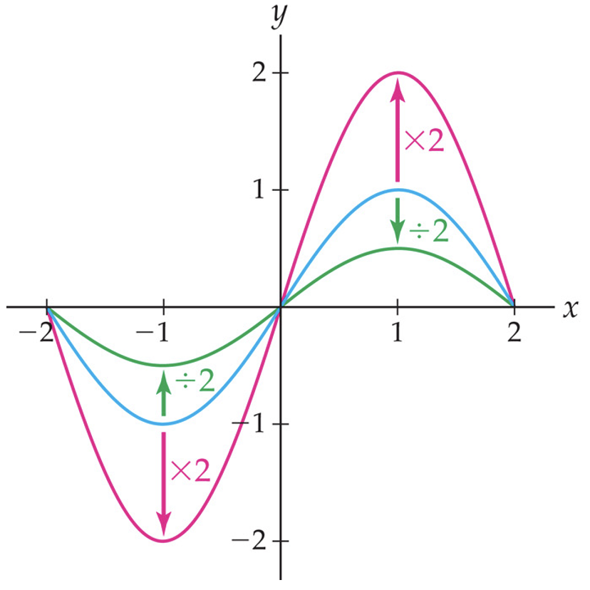
As a result, the graph of \(g\) is obtained by taking points on the graph of \(f\) and “scaling” their \(y\)-coordinates by the constant \(c\text{.}\) This has the graphical effect of vertically stretching (if \(c> 1\)) or vertically shrinking (if \(c< 1\)) the graph of \(f\text{.}\)
As a result, the graph of \(g\) is obtained by taking points on the graph of \(f\) and “scaling” their \(x\)-coordinates by the constant \(1/c\text{.}\) This has the graphical effect of horizontally stretching (if \(c< 1\)) or vertically shrinking (if \(c> 1\)) the graph of \(f\text{.}\)
Remark1.6.11.Transformations: vertical versus horizontal effects.
A clear pattern emerges from the four types of transformations we have considered. Transformations that affect the output\(f(x)\) (the “outside” of the function) have a vertical effect on the graph of the function, while transformations that affect the input\(x\) (the “inside” of the function) have a horizontal effect on the graph of the function. Furthermore, for both types of transformations, additive changes (\(+c\)) result in shifts, while multiplicative changes (\(\cdot c\)) result in stretches or shrinks.
Note also that the transformations involving the input give rise to a graphical effect that is the reverse of what you might have initially expected. For example, the transformation \(f(x)\longmapsto f(x+3)\) shifts the graph of \(f\) to the left by 3 units, not to the right. Similarly, the transformation \(f(x)\longmapsto f(2x)\) shrinks the graph of \(f\) horizontally by a factor of 2, rather than stretching it.
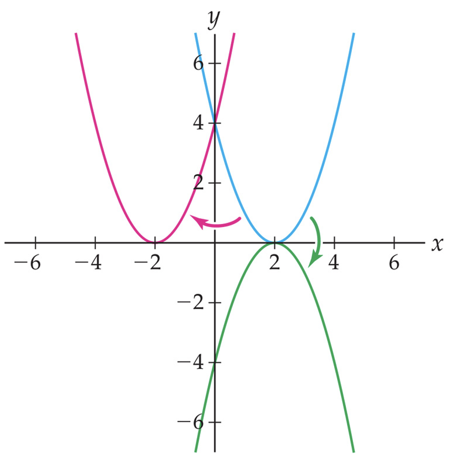
Following the same chain of logic as in the examples above we observe that a point \(P=(x,y)\) lies on the graph of \(f\) if and only if the point \(Q=(x,-y)\) lies on the graph of \(g(x)=-f(x)\text{.}\) Graphically, this means that the graph of \(g=-f(x)\) is obtained by reflecting the graph of \(f\) across the \(x\)-axis.
Similarly, a point \(P=(x,y)\) lies on the graph of \(f\) if and only if the point \(Q=(-x,y)\) lies on the graph of \(g(x)=f(-x)\text{.}\) Graphically, this means that the graph of \(g=f(-x)\) is obtained by reflecting the graph of \(f\) across the \(y\)-axis.
The first transformation reflects the graph of \(f\) across the \(y\)-axis; the second shrinks the resulting graph by a factor of two. Combined, we see that the transformation
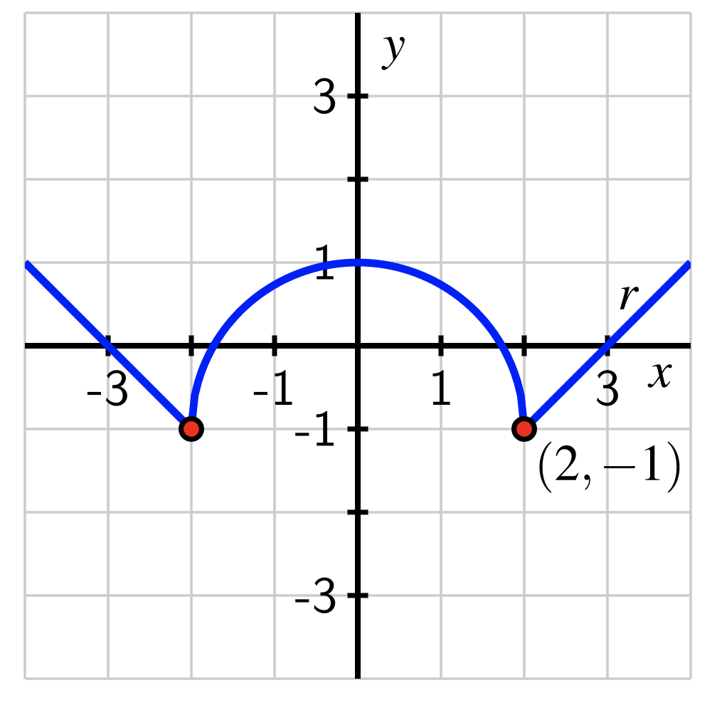
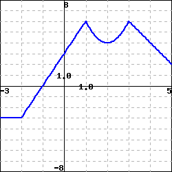
Consider the function \(r\) given in Figure 1.6.17 below. Describe in words how the function \(m(x) = 2r(x+1)-1\) is the result of three transformations of \(r(x)\text{.}\) Does the order in which these transformations occur matter? Why or why not?
There are three basic transformations involved: a vertical shift of 1 unit down, a horizontal shift of 1 unit left, and a vertical stretch by a factor of 2. To understand the order in which these transformations are applied, it’s essential to remember that a function is a process that converts inputs to outputs.
By the algebraic rule for \(m\text{,}\)\(m(x) = 2r(x+1)-1\text{.}\) In words, this means that given an input \(x\) for \(m\text{,}\) we do the following processes in this particular order:
add 1 to \(x\) and then apply the function \(r\) to the quantity \(x+1\text{;}\)
We can see the graphical impact of these algebraic steps by taking them one at a time. Note that in each of the following figures, we track the point \((2,-1)\) from the original function.
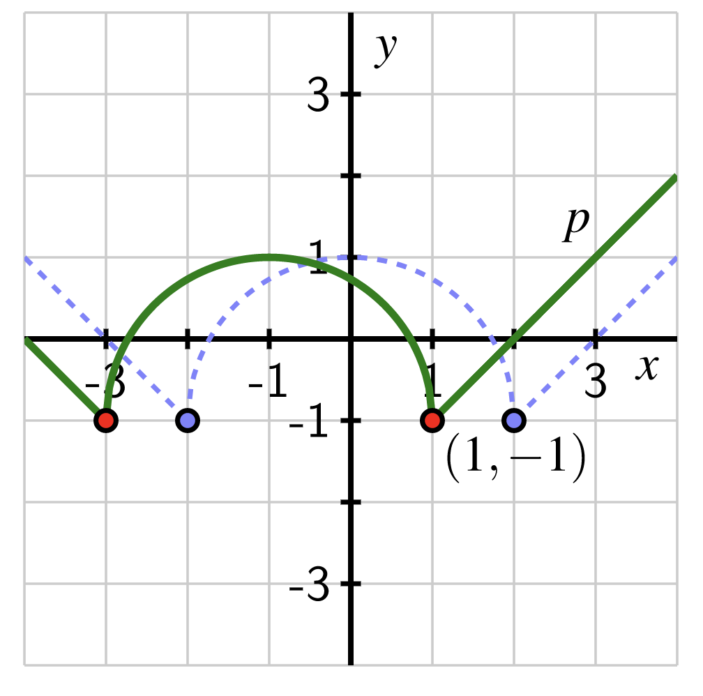
In Figure 1.6.18, we see the function that results from a shift of 1 unit left of the function \(y=r(x)\) in Figure 1.6.17. The tracked point first moves left 1 unit to \((1,-1)\text{.}\) (Each time we take an additional step, we will de-emphasize the preceding function by having it appear in lighter color and dashed.)
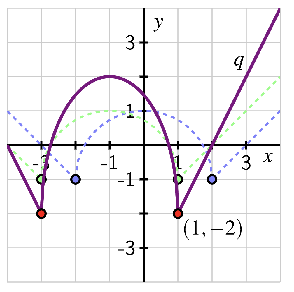
Continuing, we now consider the function \(y=2r(x+1)\text{,}\) which results in a vertical stretch away from the \(x\)-axis by a factor of 2, as seen in Figure 1.6.19. The tracked point is stretched vertically by a factor of 2 away from the \(x\)-axis to \((1,-2)\text{.}\)
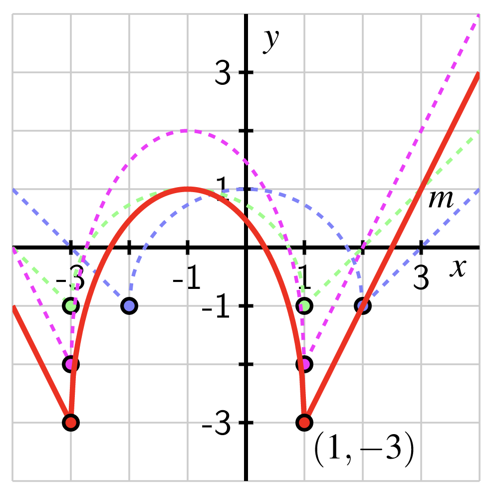
Finally, we arrive at \(y=2r(x+1)-1\) by subtracting 1 from the previous graph; this of course is a vertical shift of \(-1\) units, and produces the graph of \(m\) shown in red in Figure 1.6.20. The tracked point is shifted 1 unit down to the point \((1,-3)\text{.}\)
While there are some transformations that can be executed in either order (such as the combination of a horizontal translation and a vertical translation, in other situations order matters. In this example, we have to apply the vertical stretch before applying the vertical shift, Algebraically, this is because
The quantity \(2r(x+1)-1\) multiplies the function \(r(x+1)\) by 2 first (the stretch) and then the vertical shift follows; the quantity \(2[r(x+1)-1]\) shifts the function \(r(x+1)\) down 1 unit first, and then executes a vertical stretch by a factor of 2. In the latter scenario, the point \((1,-1)\) that lies on \(r(x+1)\) gets transformed first to \((1,-2)\) and then to \((1,-4)\text{,}\) which is not the same as the point \((1,-3)\) that lies on \(m(x)=2r(x+1)-1\text{.}\)
Checkpoint1.6.21.Vertical and horizontal translations, stretches, and reflections.
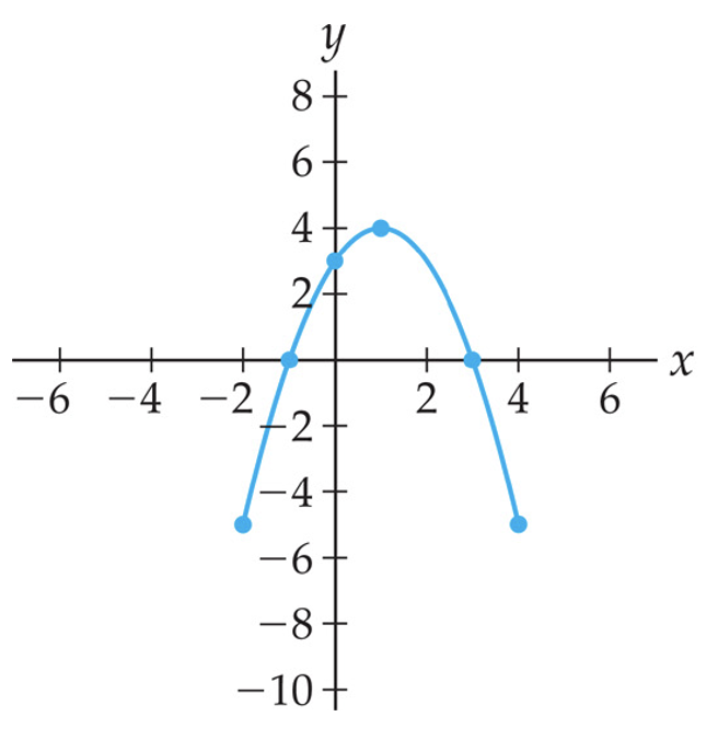
The figure that follows shows a piece of the graph of a parabola with five marked points. Sketch graphs for each of the given transformations. On each graph, mark the new coordinates of the five marked points
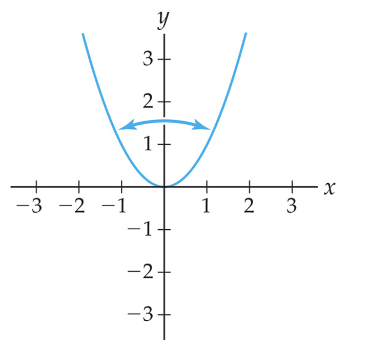
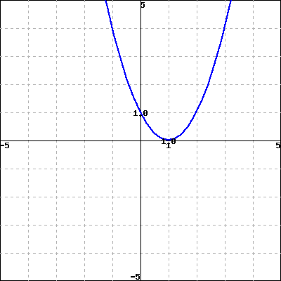
Some graphs do not change under certain transformations. For example, the graph of \(f(x) = x^2\) shown in Figure 1.6.22 below remains the same if we reflect it across the \(y\)-axis. We say that this function has \(y\)-axis reflectional symmetry.
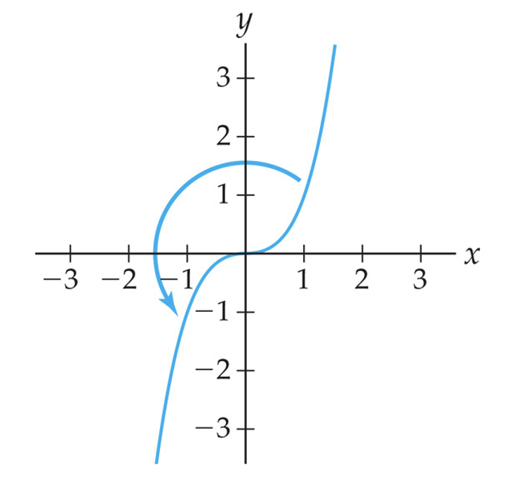
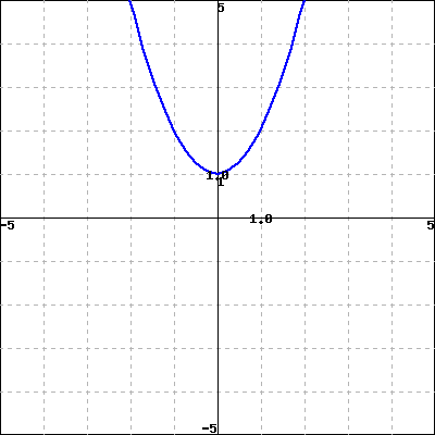
As another example, the graph of \(g(x) = x^3\) shown in Figure 1.6.23 below remains the same if we reflect it first across the \(y\)-axis and then across the \(x\)-axis. This double-reflection across the \(x\)- and \(y\)-axis is equivalent to rotation around the origin by \(180^\circ\text{.}\) Take a moment to experiment with this: on a piece of scrap paper, draw a smiley face or some other picture. Flip the paper vertically and then horizontally (or horizontally and then vertically). This gives you the same result as rotating the paper by 180 degrees. A function that is preserved under the transformation of \(180^\circ\) rotation is said to have \(180^\circ\)rotational symmetry.
These types of symmetries are also called even symmetry and odd symmetry, since power functions with even powers all have \(y\)-axis symmetry and power functions with odd powers all have rotational symmetry. Let’s try to understand algebraically what makes the graph of a function \(f\) have even or odd symmetry. The graph has even symmetry when the following equivalence holds:
\begin{equation*}
(x,y) \text{ is on the graph of } f \iff (-x,y) \text{ is on the graph of } f\text{.}
\end{equation*}
Since a point \((x,y)\) is on the graph of \(f\) if and only if \(x\) is in the domain of \(f\) and \(f(x)=y\text{,}\) we see that the above equivalence is equivalent to the algebraic statement
\begin{equation*}
f(-x)=f(x)
\end{equation*}
for all \(x\) in the domain of \(f\text{.}\) Similarly, the graph of \(f\) has odd symmetry if and only if \(f(x)=-f(x)\) for all \(x\) in its domain. This is the motivation for the following definition and table.
Observe the technical restriction placed on the domain of a function in Definition 1.6.24. Namely, we do not even ask whether a function \(f\colon D\rightarrow \R\) is even or odd, if its domain \(D\) does not satisfy the property
For example, \(n\)-th root functions \(f(x)=\sqrt[n]{x}\) for \(n\) even are not possible candidates for evenness or oddness, since their domain \(D=[0,\infty)\) does not satisfy this property: e.g., \(1\in D\text{,}\) but \(-1\notin D\text{.}\)
It should be noted that being even or odd is a special property not enjoyed by all functions. In fact, chances are, if you write down a random algebraic function, it will be neither even nor odd.
The argument used to show that a function is not even (or not odd), is qualitatively very different than for showing the function is even (or is odd). Namely, to show the property in question does not hold, it suffices to find a single explicit counterexample. The next example illustrates this.
First observe that the implied domain of \(h\) is \(\R\text{,}\) since \(f\) is a polynomial. To show \(f\) is not even, it suffices to show that \(f(-x)\ne f(x)\) for some element \(x\in \R \text{.}\) This is easy: we have
Similarly, to show \(f\) is not odd, we need only find an iput \(x\) satisfying \(f(-x)\ne -f(x)\text{.}\) The same input \(x=1\) works in this case as well, since \(f(-1)\ne -f(1) \text{.}\)
Sketch a graph that has neither \(y\)-axis symmetry nor \(180^\circ\) rotational symmetry. Congratulations! You have drawn the graph of a function that is neither even nor odd.
Example 1.6.27 illustrates the important role played by the “for all” quantifier in Definition 1.6.24. A function is even (or odd) if it satisfies the relevant equation for all elements in its domain; and it is not even (or not odd) if it fails to satisfy the relevant equation for some element in its domain. In essence, being even or odd is a function equality statement involving the two functions \(f(x)\) and \(g(x)=f(-x)\text{:}\)\(f\) is even if \(f=g\) (as functions); and \(f\) is odd if \(f=-g\) (as functions). (See Definition 1.5.24.)
Comparing the formulas for \(f\) and \(g\text{,}\) it seems clear that these two functions are not equal, and hence that \(f\) is not even. But we need to be careful here! As we have seen before, different formulas can sometimes be seen to define the same function after some algebra. The surefire way of showing two functions are not equal is find a single instance of an input where their outputs differ. This is exactly what we did in the solution to Example 1.6.27.
In this particular case, however, we are aided by the fact that all the functions involved are polynomials, and that polynomial equality is equivalent to having like coefficients. (See Corollary 1.5.26.) That is, we can immediately see that the three functions
are distinct simply by comparing their coefficients. It follows that \(f\) is not even (since \(f(-x)\ne f(x)\)) and \(f\) is not odd (since \(-f(-x)\ne f(x)\)).
Of course, not all functions are polynomials, and so things are not always this straightforward. When in doubt, to definitely show a function is not even (or not odd), provide an explicit counterexample.
for all \(x\in D\text{,}\) we see that \(f\) is odd. Looking at the formulas, it seems clear that \(f(-x)\ne f(x)\) for all \(x\in D\text{,}\) and hence that \(f\) is not even. To be sure, however, we provide a counterexample: we have \(f(1)=1/1=1\) and \(f(-1)=1/(-1)=-1\text{.}\) Since \(f(1)\ne f(-1)\text{,}\) we conclude that \(f\) is not even.
Is \(g\) odd? In this case since \(g(x)=x^4-x^2\) and \(-g(-x)=-x^4+x^2\) are both polynomials, we see that the two functions are not equal simply by comparing coefficients. Thus \(g\) is not odd.
for all \(x\in \R\text{.}\) Looking just at the formulas, it seems that the function \(h(-x)\) is equal neither to \(h(x)\) nor \(-h(x)\text{.}\) To be sure, however, we provide explicit counterexamples to both evenness and oddness.
Note that \(h(1)=3/2\) and \(h(-1)=1/2\text{.}\) Since \(h(1)\ne h(-1)\text{,}\) we conclude that \(h\) is not even. Furthermore, since \(h(1)\ne -h(-1)\text{,}\) we conclude that \(h\) is not odd.
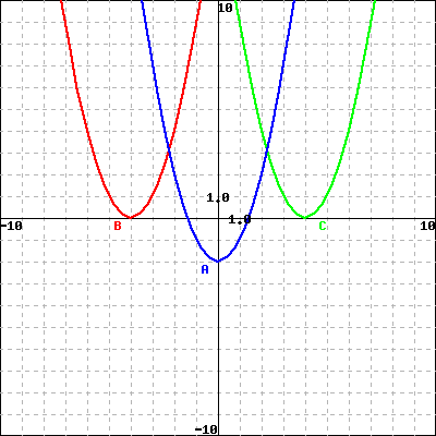
Looking at the graphs of \(f\text{,}\)\(g\text{,}\) and \(h\text{,}\) in Figure 1.6.31, we can confirm our conclusions above immediately: the graph of \(f\) exhibits \(180^\circ\) rotational symmetry, but not \(y\)-axis reflectional symmetry; the graph of \(g\) exhibits \(y\)-axis reflectional symmetry, but not \(180^\circ\) rotational symmetry; and the graph of \(h\) exhibits neither type of symmetry.
Recall that every quadratic function \(g(x)=ax^2+bx+c\) can be expressed in vertex form as \(g(x)=a(x+d)^2+e\) for some constants \(d\) and \(e\text{.}\) This result, along with our newfound understanding of function transformations, allows us to relate the graph of \(g(x)=a(x+d)^2+e\) to the graph of the simple power function \(f(x)=x^2\text{.}\) Indeed, applying the sequence of transformations
As a result, the graph of an arbitrary quadratic function can be obtained from the graph of \(f(x)=x^2\) by performing a horizontal shift, followed by a vertical scaling, followed by a vertical shift. Figure 1.6.32 illustrates this process for the function \(g(x)=-2(x-1)+3\text{.}\)
To obtain a new graph, stretch the graph of a function \(f(x)\) vertically by a factor of 7. Then shift the new graph 4 units to the right and 9 units up. The result is the graph of a function
\begin{equation*}
g(x) = A f(x+B) +C
\end{equation*}
where \(A\text{,}\)\(B\text{,}\)\(C\) are certain numbers. What are \(A\text{,}\)\(B\text{,}\) and \(C\text{?}\)
The figure above is the graph of the function \(m(t)\text{.}\) Let \(n(t)=m(t)+2\text{,}\)\(k(t)=m(t+1.5)\text{,}\)\(w(t)=m(t-0.5)-2.5\) and \(p(t)=m(t-1)\text{.}\) Find the values of the following:
The graph of \(f(x)\) contains the point \((-9, 4)\text{.}\) What point must be on each of the following transformed graphs? Enter points as \((a,b)\) including the parentheses.