Section 1.2 Linear and quadratic functions

Subsection Learning Goals

  • Understand the definition of linear and quadratic functions.
  • Explore how the parameters of a linear or quadratic function change the shape of its graph and its properties.
  • Use the different forms for equations for lines.
  • Solve quadratic equations via factoring or the quadratic formula.

Subsection Definitions of linear and quadratic functions

Part of our exploration of functions in this course will include the study of important families of functions. In this section we introduce two such families: linear functions and quadratic functions. These functions will serve as a useful starting point for two reasons: on the one hand, they are fairly simple functions and hence easy to analyze; on the other hand, these functions are widely used in real-world applications. For example, in statistics, the method of linear regression seeks to find a line that best describes the relationship between quantities that appear to change at a constant rate relative to each other; and quadratic functions are used in mechanics to model the height of an object falling under the force of gravity. We will explore several models that use linear and quadratic functions in SectionΒ 1.3 after we develop our mathematical understanding of them.
We begin with the mathematical definitions of linear and quadratic functions. Recall that a mathematical definition is "used to give a precise meaning to a new term, by describing a condition which unambiguously qualifies what a mathematical term is and is not."
 2 
Thus the definitions below give us the precise meaning of a linear or quadratic function. Remember that we generally need a few examples to make sense of definitions, and these follow below each of the definitions.

Definition 1.2.2. Linear functions.

A function \(f\) is linear (or affine) if there are real constants \(m\) and \(b\) such that
\begin{equation} f(x)=mx+b\tag{1.11} \end{equation}
for all \(x\) in its domain.

Example 1.2.3. Linear functions.

Verify that the given function is linear using DefinitionΒ 1.2.2.
  1. \(\displaystyle f(x)=3x+1\)
  2. \(\displaystyle g(t)=t\)
  3. \(\displaystyle h(s)=1.2\)
  4. \(\displaystyle f(x)=\frac{1}{2}(x+2)+2x+1\)
Solution.
  1. It follows immediately that \(f\) is linear. Here \(m=3\) and \(b=1\text{.}\)
  2. We have
    \begin{equation*} g(t)=t=1\cdot t+0 \end{equation*}
    for all \(t\) in the domain of \(g\text{.}\) Thus \(g\) is linear with \(m=1\) and \(b=0\text{.}\)
  3. We have
    \begin{equation*} h(s)=1.2=0\cdot s+1.2\text{.} \end{equation*}
    Thus \(h\) is linear with \(m=0\) and \(b=1.2\text{.}\)
  4. We have
    \begin{equation*} f(x)=\frac{1}{2}(x+2)+2x+1=\frac{1}{2}x+1+2x+1=\frac{5}{2}x+2 \end{equation*}
    for all \(x\text{.}\) Thus \(f\) is linear with \(m=\frac{5}{2}\) and \(b=2\text{.}\)

Remark 1.2.4. Standard form.

As illustrated by ExampleΒ 1.2.3, a function can be linear even if its given formula does not look precisely like the form in (1.11). Often we need to manipulate the given formula algebraically in order to bring it into the standard form prescribed by (1.11).
ExampleΒ 1.2.3 included to important types of linear functions that deserve their own definition: the identity function and constant functions.

Definition 1.2.5. Identity function and constant functions.

  • A function \(f\) is an identity function if
    \begin{equation} f(x)=x\tag{1.12} \end{equation}
    for all \(x\) in its domain.
  • A function \(f\) is a constant function if there is a real constant \(c\) such that
    \begin{equation} f(x)=c\tag{1.13} \end{equation}
    for all \(x\) in its domain.
We now move on to quadratic functions, which are only slightly more complicated than linear functions.

Definition 1.2.6. Quadratic function.

A function \(f\) is quadratic if there are real constants \(a,b,c\) with \(a\ne 0\) such that
\begin{equation} f(x)=ax^2+bx+c\tag{1.14} \end{equation}
for all \(x\) in its domain.

Remark 1.2.7. Quadratic functions.

Why do we insist that \(a\ne 0\) in DefinitionΒ 1.2.6? This is to distinguish linear functions as a separate family from quadratic functions. If we allowed \(a=0\) in our definition of quadratic functions then a linear function \(f(x)=mx+b\) would also be quadratic, since
\begin{equation*} f(x)=mx+b=0x^2+mx+b \end{equation*}
for all \(x\) in its domain.
As with linear functions, we sometimes need to do a little algebraic work to show that a given quadratic function has a formula of the standard form represented by (1.14).

Checkpoint 1.2.8.

Verify that the given function is quadratic using DefinitionΒ 1.2.6.
  1. \(\displaystyle f(x)=(x-2)^2\)
  2. \(\displaystyle g(x)=x^3-x(x^2+3x-7)+2\)
  3. \(\displaystyle h(t)=t^2\)
Solution.
  1. We have
    \begin{align*} f(x) \amp =(x-2)^2\\ \amp = x^2-4x+4\text{,} \end{align*}
    showing that \(f\) is quadratic.
  2. We have
    \begin{align*} g(x) \amp= x^3-x(x^3+3x-7)+2 \\ \amp = x^3-x^3-3x^2+7x+2\\ \amp =-3x^2+7x+2\text{.} \end{align*}

Remark 1.2.9. Parameters.

It is important to note that when we write an expression like \(f(x) = mx+b\) or \(f(x) = ax^2+bx+c\text{,}\) only \(x\) is being treated as a variable. The extra letters \(a, b, c\text{,}\) and \(m\) that are not variables are called parameters of the function. How should you think about these parameters and what they represent?
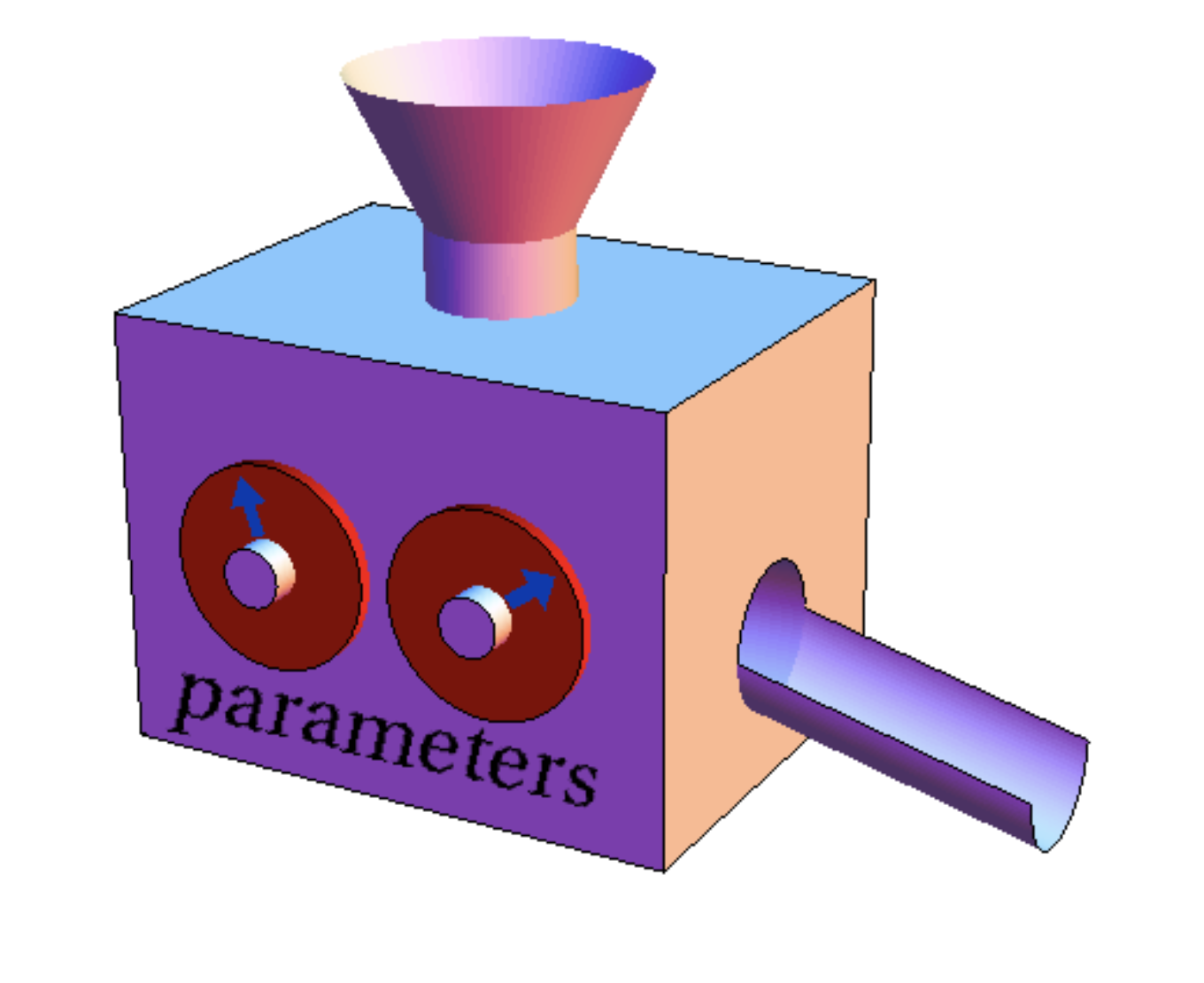
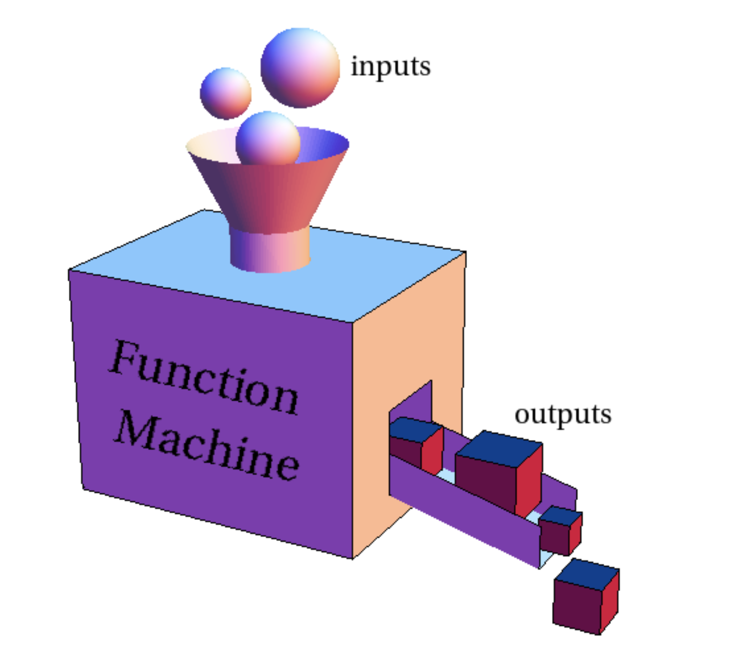
While the word parameter may be new to you, the concept is probably not so unfamiliar. We can think of a parameter as a "dial" on the function machine. Setting the dials to different values creates different functions.
 3 
(a) Function visualized as machine turning inputs into outputs
(b) Parameters visualized as adjustment dials on function machine
Figure 1.2.10. Machine analogy for functions and parameters
Consider the general form of a linear function:
\begin{equation*} f(x) = mx + b\text{.} \end{equation*}
Here \(x\) is the independent variable that is allowed range over all elements of the domain of \(f\text{,}\) whereas the constants \(m\) and \(b\) are parameters.
  • If we choose a specific value of \(m\) and \(b\) (β€œset the dials”), we get a specific function. For example, if \(m = 3\) and \(b = -7\) we get the linear function \(f(x)= 3x - 7\text{.}\)
  • As we change the parameters \(m\) and \(b\) (β€œadjusting the dials”), we get different linear functions with different properties.
Thus, when we give a general form of a linear function \(f(x)=mx+b\) in terms of unspecified parameters \(m\) and \(b\text{,}\) we are really presenting an entire family of functions: we get one linear function for each choice of the parameter values \(m\) and \(b\text{.}\)

Example 1.2.11. Desmos: family of linear functions.

The Desmos interactive in FigureΒ 1.2.12 illustrates what effect the parameters \(m\) and \(b\) defining a linear function have on the graph of this function.
  1. Play around with the values of \(m\) and \(b\text{.}\) Identify what graphical property each parameter represents.
  2. Can you find values of \(m, b\) that represents a horizontal line? Can you find values of \(m, b\) that represents a vertical line? If so, what are they? If not, why not?
Figure 1.2.12. Desmos interactive: adjusting parameters of linear functions
Similarly, the general form
\begin{equation*} f(x)=ax^2+bx+c \end{equation*}
of a quadratic function gives rise to an entire family of functions, one for each choice of the parameters \(a,b,c\text{.}\) The graphical effect of these parameters on a quadratic function is explored in ExampleΒ 1.2.13. As you will see, the relationship between the parameters and the graph is not as straightforward as it is for linear functions.

Example 1.2.13. Desmos: family of quadratic functions.

The Desmos interactive in FigureΒ 1.2.14 explores what effect the parameters \(a,b,c\) have on the graph of a quadratic function of the form \(f(x)=ax^2+bx+c\text{.}\)
  1. Note that the graphs of quadratic functions are always parabolas. What detail about the parameters \(a,b,c\) determines whether this parabola opens up or down?
  2. How does the parameter \(c\) affect the graph of the function?
Figure 1.2.14. Desmos interactive: adjusting parameters of quadratic functions

Subsection Properties of linear functions

Before drilling down more in our analysis of linear and quadratic functions, we give a formal definition of various properties of functions that we will be interested in studying.

Definition 1.2.15. Properties of functions.

Let \(f\) be a function with domain \(D\subseteq \R\text{.}\)
  • Zeros and \(x\)-intercepts.
    A zero (or root) of \(f\) is an element \(c\in D\) satisfying \(f(c)=0\text{.}\) An \(x\)-intercept of \(f\) is a point on the graph of \(f\) of the form
    \begin{equation*} (c,0)=(c,f(c))\text{.} \end{equation*}
    Thus each zero \(c\) of \(f\) gives rise to an \(x\)-intercept \((c,0)\) on the graph of \(f\text{,}\) and vice versa. Graphically speaking, an \(x\)-intercept is a point where the graph of \(f\) intersects the \(x\)-axis.
  • \(y\)-intercept.
    Assume \(0\in D\text{.}\) The \(y\)-intercept of \(f\) is the point
    \begin{equation*} (0,f(0)) \end{equation*}
    on the graph of \(f\text{.}\) Graphically speaking, the \(y\)-intercept is the point where the graph of \(f\) intersects the \(y\)-axis.
  • Positive/negative.
    Let \(I\subseteq D\) be an interval. We say \(f\) is positive (resp., negative) on \(I\text{,}\) denoted \(f> 0\) (resp., \(f< 0\)), if \(f(x)> 0\) (resp., \(f(x)< 0\)) for all \(x\in I\text{.}\) Similarly, \(f\) is nonnegative (resp. nonpositive) on \(I\text{,}\) denoted \(f\ge 0\) (resp., \(f\le 0\)), if \(f(x)\ge 0\) (resp., \(f(x)\le 0\)) for all \(x\in I\text{.}\)
    Graphically speaking, \(f\) is positive on \(I\) if points \((x,f(x))\) of \(f\) lie above the \(x\)-axis for all \(x\in I\text{.}\) Similar statements apply for negative, nonnegative, and nonpositive.
  • Increasing/decreasing.
    Let \(I\subseteq D\) be an interval. We say \(f\) is increasing on \(I\) if for all \(a,b\in D\text{,}\) if \(a< b\text{,}\) then \(f(a)< f(b)\text{.}\) Similarly, we say \(f\) is decreasing on \(I\) if for all \(a,b\in D\text{,}\) if \(a< b\text{,}\) then \(f(a)> f(b)\text{.}\)
    Graphically speaking, if \(f\) is increasing (resp. decreasing) on \(I\) then the graph of \(f\) moves up (resp. down) as we move to the right.
  • Maximum/minimum.
    Let \(D'\subseteq D\) and let \(c\in D'\text{.}\) We say \(f\) has a maximum at \(c\) relative to \(D'\) if \(f(c)\ge f(x)\) for all \(x\in D'\text{.}\) In this case we call \(f(c)\) the maximum value of \(f\) on \(D'\text{.}\) Similarly, we say \(f\) has a minimum at \(c\) relative to \(D'\) if \(f(c)\le f(x)\) for all \(x\in D'\text{,}\) and in this case we call \(f(c)\) the minimum value of \(f\) on \(D'\text{.}\)
    A maximum (resp. minumum) \(c\) of \(f\) relative to the entire domain \(D\) is called a global maximum (resp. global minimum) of \(f\text{,}\) and in this case \(f(c)\) is called the global maximum value (resp. global minimum value) of \(f\text{.}\)
    Graphically speaking, \(f\) has a maximum (resp., minimum) at \(c\in D'\) if the point \((c,f(c))\) is the highest (resp., lowest) point on the graph of \(f\) with \(x\)-coordinate in \(D'\text{.}\)
Let’s test out some of this new terminology on some linear functions.

Example 1.2.16. Linear function properties.

For the given function \(f\colon \R\rightarrow \R\) do the following: (a) find all \(x\)- and \(y\)-intercepts, (b) determine the intervals on which \(f\) is positive, negative, increasing, and decreasing, (c) find all inputs where \(f\) has a global maximum or minumum (if any). The Desmos interactive in FigureΒ 1.2.12 may be helpful.
  1. \(\displaystyle f(x)=-2x+3\)
  2. \(\displaystyle f(x)=3x+5\)
  3. \(\displaystyle f(x)=-2\)
Graph of f(x)=-2x+3
(a) Graph of \(f(x) = -2x + 3\)
Graph of f(x)=3x+5
(b) Graph of \(f(x) = 3x + 5\)
Graph of f(x)=-2
(c) Graph of \(f(x) = -2\)
Figure 1.2.17. Three linear functions
Solution.
  1. The \(y\)-intercept of \(f\) is easily computed as
    \begin{equation*} (0,f(0))=(0,3)\text{.} \end{equation*}
    To find the \(x\)-intercept(s) of \(f\text{,}\) we solve the equation \(f(x)=0\text{:}\)
    \begin{align*} f(x) \amp = 0\\ -2x+3 \amp = 0\\ -2x \amp = -3\\ x \amp = \frac{3}{2}\text{.} \end{align*}
    We conclude that \(f\) has exactly one zero (or root), \(x=3/2\) and hence exactly only \(x\)-intercept, \((3/2,0)\text{.}\)
    Looking at the graph of \(f(x)=-2x+3\text{,}\) we see that the function is decreasing on every interval \(I\subseteq \R\text{:}\) in plain English, the graph of \(f\) always moves down as we move to the right.
    Since \(f\) has a unique zero at \(x=3/2\) and is decreasing on \(\R\text{,}\) it follows that \(f\) is positive on the interval \((-\infty,3/2)\) and negative on the interval \((3/2,\infty)\text{.}\)
    Moreover, it follows from \(f\) being decreasing on \(\R\) that it has no global maximum or minimum value. Roughly speaking, given any input \(c\text{,}\) the value of \(f\) will be greater than \(f(c)\) for inputs to the left of \(c\text{,}\) and less than \(f(c)\) for inputs to the right. More formally, if we choose any \(a\in \R\) with \(a< c\text{,}\) then since \(f\) is decreasing everywhere we have \(f(a)> f(c)\text{;}\) similarly, if we choose any \(b\in \R\) with \(b> c\text{,}\) we have \(f(b)< f(c)\text{.}\) Thus \(f\) has neither a global maximum nor global minimum at \(c\text{.}\) Since \(c\) was arbitrary, there is no input where \(f\) has a global maximum or minimum.
  2. Reasoning along the same lines as in (a), we find that the \(y\)-intercept of \(f\) is
    \begin{equation*} (0,f(0))=(0,5) \end{equation*}
    and there is a unique \(x\)-intercept at
    \begin{equation*} (-\frac{5}{3},0) \end{equation*}
    corresponding to the unique solution of the equation \(3x+5=0\text{.}\)
    Moreover, the function \(f\) is increasing on every interval \(I\subseteq \R\text{,}\) from whence it follows that \(f\) is negative on the interval \((-\infty,-\frac{5}{3})\) and positive on the interval \((-\frac{5}{3},\infty)\text{.}\)
    Lastly, since \(f\) is increasing on \(\R\text{,}\) it follows that \(f\) has no global maximum or minimum value, and thus no input where it has a global maximum or minimum.
  3. Our answers for the constant function \(f(x)=-2\) are qualitatively very different from those in (a) and (b). As always, the \(y\)-intercept of \(f\) is easily computed as
    \begin{equation*} (0,f(0))=(0,-2)\text{,} \end{equation*}
    since \(f(x)=-2\) for all inputs \(x\in \R\text{.}\) However, in this case there are no \(x\)-intercepts. Algebraically, this is a result of the fact that \(f(x)=-2\) for all \(x\in \R\text{,}\) and hence that we cannot have \(f(x)=0\) for any \(x\in \R\text{.}\) Graphically, this is reflected in the fact that the graph of \(f\text{,}\) the horizontal line \(y=-2\text{,}\) does not intersect the \(x\)-axis.
    Since the value of \(f\) is equal to \(-2\) for all inputs, we see that \(f\) is always negative and never positive. Furthermore, over any interval \(I\subseteq \R\text{,}\) since the value of \(f\) on \(I\) is constant, it is neither increasing nor decreasing. Finally, we see that \(-2\) is both the global maximum and global minimum value of \(f\text{:}\) a trivial result of its being the only value of \(f\text{!}\) Since \(f(x)=-2\) for all \(x\in \R\text{,}\) it follows that \(f\) has a global maximum and global minimum at every element in its domain!
Our analysis of the three linear functions in ExampleΒ 1.2.16 easily generalizes to the family of all linear functions, as we now make official.
As illustrated by all of our examples, the graph of a linear function is a line in \(\R^2\text{.}\) Why is this so? Recall from our discussion in Vertical line test that the graph of the function \(f(x)=mx+b\) is the same thing as the graph of the equation
\begin{equation*} y=mx+b\text{,} \end{equation*}
which we recognize as the slope-intercept form of the equation of a line. In DefinitionΒ 1.2.19 we recall some of the different forms of equations of lines in the plane.

Definition 1.2.19. Equations of lines.

Let \(L\) be a line in the plane \(\R^2\text{.}\)
A general form of \(L\) is any equation of the form
\begin{equation} ax+by=c\text{,}\tag{1.15} \end{equation}
where \(a\text{,}\) \(b\text{,}\) and \(c\) are real constants, and \(L\) is the graph of (1.15). Every line in the plane has a general form.
Assume now that \(L\) is not a vertical line.
  • Slope.
    The slope of \(L\) is the constant \(m\) defined as
    \begin{equation} m=\frac{y_2-y_1}{x_2-x_1}\text{,}\tag{1.16} \end{equation}
    where \(P_1=(x_1,y_1)\) and \(P_2=(x_2,y_2)\) are any two distinct points on \(L\text{.}\)
  • Point-slope form.
    A point-slope form of \(L\) is an equation of \(L\) of the form
    \begin{equation} y-y_0=m(x-x_0)\text{,}\tag{1.17} \end{equation}
    where \(P=(x_0,y_0)\) is any point on \(L\text{,}\) and \(m\) is the slope of \(L\text{.}\)
  • Slope-intercept form.
    The slope-intercept form of \(L\) is the unique equation of \(L\) of the form
    \begin{equation} y=mx+b\text{,}\tag{1.18} \end{equation}
    where \(m\) is the slope of \(L\) and \(b\) is a constant.

Remark 1.2.20. Equations of lines.

As suggested by DefinitionΒ 1.2.19, a line \(L\) in \(\R^2\) does not have a single defining equation, but rather many different equations of varying form. Some comments are in order.
  • The general form of a line is useful theoretically, as any line in \(\R^2\) can be defined in this manner. In particular, vertical lines, have defining equations in general form (namely, \(x=c\)), but no defining equation in slope-intercept or point-slope form.
  • The slope \(m\) of a line is only defined for non-vertical lines. The fact that it can be computed as
    \begin{equation*} m=\frac{y_2-y_1}{x_2-x_1}\text{,} \end{equation*}
    where \(P_1=(x_1,y_1)\) and \(P_2=(x_2,y_2)\) are any two distinct points on \(L\) is evidence of a certain regularity that lines satisfy. Indeed, letting \(\Delta y=y_2-y_1\) and \(\Delta x=x_2-x_1\text{,}\) we see that
    \begin{equation*} m=\frac{\Delta y}{\Delta x} \end{equation*}
    is the ratio of the change in \(y\) to the change in \(x\) between any two points on \(L\text{.}\) The fact that this ratio does not depend on the choice of points means that starting from any point \(L\text{,}\) as we move to the right on \(L\) any positive distance \(\Delta x\text{,}\) we move vertically by a directed distance of
    \begin{equation*} \Delta y=m\cdot \Delta x\text{.} \end{equation*}
    We summarize this observation by saying that the slope computes the "rise over run" of the line \(L\text{:}\)
    \begin{equation} m=\frac{\Delta y}{\Delta x}=\frac{\text{ rise } }{\text{ run } }\text{.}\tag{1.19} \end{equation}
  • The slope-intercept form \(y=mx+b\) of a non-vertical line \(L\) is useful, as we can read off the slope \(m\) and \(y\)-intercept \((0,b)\) directly from the equation. Furthermore, unlike the other equation forms of a line, the slope-intercept form is unique. As a consequence, we can distinguish two lines simply by looking at their slope-intercept forms (assuming both lines are non-vertical).
  • By contrast, the point-slope form \(y-y_0=m(x-x_0)\) of a non-vertical line \(L\) is not unique. Indeed, though the parameter \(m\) appearing in such an equation is unique (being the slope of the line), the constants \(x_0\) and \(y_0\) are not unique since they can be chosen as the \(x\)- and \(y\)- coordinates of any point on the line.
    That said, it is precisely this non-uniqueness that makes the point-slope form so useful. As illustrated in ProcedureΒ 1.2.21, as soon as we know the slope of a line and the coordinates of any point on the line, we can derive a point-slope form. Furthermore, if desired, we can always easily derive the slope-intercept form from the point-slope form using a little algebra. (See ProcedureΒ 1.2.21.)
Two common ways of specifying a line \(L\) in \(\R^2\) is either by specifying its slope and providing a point, or by specifying two distinct points on \(L\text{.}\) The procedure below describes how to derive a point-slope form of the line in each of these situations.

Example 1.2.22. Equations of lines.

Find both a point-slope form and the slope-intercept form for the given line. Recall that two lines in parallel in \(\R^2\) if and only if they have the same slope, and perpendicular if and only if their slopes are negative reciprocals of each other.
  1. \(L\) is the line with slope \(-2\) that passes through the point \((3,1)\text{.}\)
  2. \(L\) is the line that passes through the points \((-1, 2)\) and \((3,4)\text{.}\)
  3. \(L\) is the line passing through \((4,9)\) that is parallel to the line \(2x-3y=5\text{.}\)
  4. \(L\) is the line that passes through the point \((2,0)\) and is perpendicular to the line \(y=\frac{1}{3}x+1\text{.}\)
Solution.
  1. Using the point-slope formula with slope \(m=-2\) and point \((3,1)\text{,}\) we get the equation \(y = -2(x-3)+1\text{.}\) To derive the slope-intercept form, we simply distribute:
    \begin{equation*} y = -2(x-3)+1=-2x+6+1=-2x+7\text{.} \end{equation*}
  2. The slope of the line through the points \((x_1,y_1) = (-1,2)\) and \((x_2,y_2) =(3,4)\) is
    \begin{equation*} m=\frac{y_2-y_1}{x_2-x_1} = \frac{4-2}{3-(-1)} =\frac{2}{4} = \frac{1}{2}\text{.} \end{equation*}
    From the slope \(m\) and the point \((-1,2)\) we derive the point-slope form
    \begin{equation*} y-2=m(x-(-1))=\frac{1}{2}(x+1)\text{.} \end{equation*}
    We then derive the slope-intercept form as
    \begin{equation*} y=\frac{1}{2}(x+1)+2=\frac{1}{2}x+\frac{1}{2}+2=\frac{1}{2}x+\frac{5}{2}\text{.} \end{equation*}
    Note that using the other point \((3,4)\) would yield a different point-slope form
    \begin{equation*} y-4=\frac{1}{2}(x-3)\text{,} \end{equation*}
    which can then be brought into the same slope-intercept form as above with a little algebra.
  3. The line with equation \(2x-3y=5\) can be rewritten in slope-intercept form as
    \begin{equation*} y=\frac{2}{3}x-\frac{5}{3}\text{,} \end{equation*}
    and thus has slope \(\frac{2}{3}\text{.}\) Since the line \(L\) is parallel to this line it also has slope \(\frac{2}{3}\text{.}\) Since it passes through the point \((4,9)\text{,}\) \(L\) has point-slope form
    \begin{equation*} y-9=\frac{2}{3}(x-4)\text{,} \end{equation*}
    and thus slope-intercept form
    \begin{equation*} y=\frac{2}{3}(x-4)+9=\frac{2}{3}x-\frac{8}{3}+\frac{27}{3}=\frac{2}{3}x+\frac{19}{3}\text{.} \end{equation*}
  4. The line we are looking for is perpendicular to \(y=\frac{1}{3}x+1\) and thus has slope \(m=-\frac{1}{1/3} = -3\text{.}\) Using the point-slope form with slope \(m=-3\) and point \((x_0,y_0)=(2,0)\text{,}\) we obtain the equation
    \begin{equation*} y=-3(x-2)\text{.} \end{equation*}
    As above, a little algebra then reveals the slope-intercept form
    \begin{equation*} y=-3x+6\text{.} \end{equation*}

Remark 1.2.23. Checking the Answer.

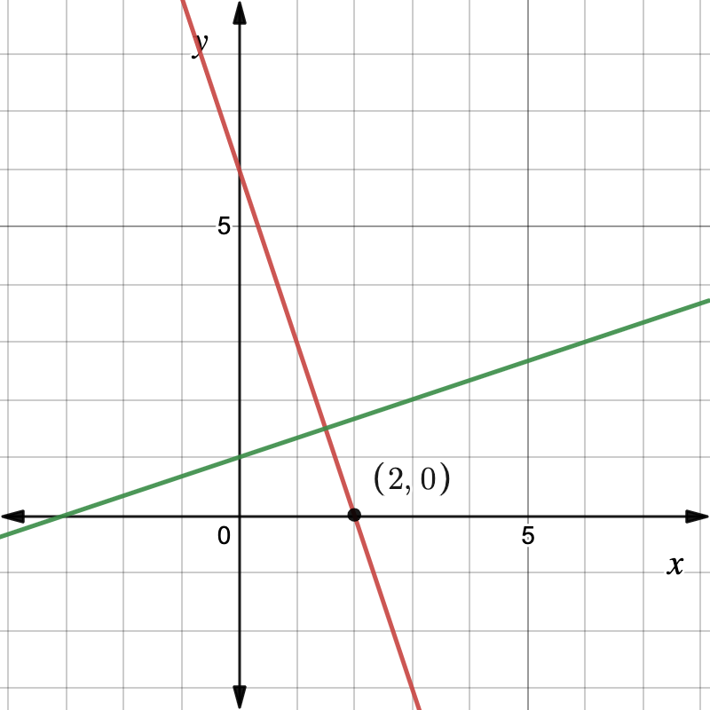
To verify that the three linear functions we just found are reasonable, we can graph them with a graphing utility (such as Desmos). In particular, let’s graph the lines \(y=-3x+6\) (red) and \(y=\frac{1}{3}x+1\) (green) in part c to make sure they appear to be perpendicular:
Notice that the scales on the \(x\)- and \(y\)-axes are the same, so the lines correctly appear as perpendicular. Additionally, we can see that the point \((2,0)\) is on the line \(y=-3x+6\text{.}\)

Subsection Vertex form

In exploring properties of quadratic functions, we are naturally led to two useful algebraic techniques: solving quadratic equations (by factoring or using the quadratic formula) and completing the square.
Given a quadratic function of the form \(f(x)=ax^2+bx+c\text{,}\) in order to find its roots and \(x\)-intercepts, we need to solve the equation
\begin{equation*} ax^2+bx+c=0\text{.} \end{equation*}
ProcedureΒ 1.2.29 describes a systematic procedure for solving such equations. The validity of that technique relies on two important results about real number algebra that are deserving of their own official statements.

Remark 1.2.25. Logical notation.

The previous theorem sneaks in an important notion from logic, the β€œif and only if” connector, along with its double-headed, double-barreled arrow notation \(\iff\text{.}\) In general, given propositions \(\mathcal{P}\) and \(\mathcal{Q}\text{,}\) the compound statement β€œ\(\mathcal{P}\) if and only if \(\mathcal{Q}\)”, written using logical notation as
\begin{equation*} \mathcal{P}\iff \mathcal{Q} \end{equation*}
means that proposition \(\mathcal{P}\) is true exactly when proposition \(\mathcal{Q}\) is true. More formally, this means the statements are logically equivalent.
Logical equivalence, along with its logical notation \(\iff\text{,}\) is intimately related to the notion of logical implication, and its notation \(\implies\text{.}\) The statement β€œ\(\mathcal{P}\) implies \(\mathcal{Q}\)” or β€œif \(\mathcal{P}\text{,}\) then \(\mathcal{Q}\)”, written
\begin{equation*} \mathcal{P}\implies \mathcal{Q}\text{,} \end{equation*}
is the assertion that if proposition \(\mathcal{P}\) is true, so is proposition \(\mathcal{Q}\text{.}\)
Mark well that the logical equivalence statement \(\mathcal{P}\iff \mathcal{Q}\) is stronger than the logical implication statement \(\mathcal{P}\implies \mathcal{Q}\text{.}\) More precisely, to assert \(\mathcal{P}\iff \mathcal{Q}\) is equivalent to asserting that two implications hold: \(\mathcal{P}\implies \mathcal{Q}\) and \(\mathcal{Q}\implies \mathcal{P}\text{.}\) This exlains why we use the double-headed arrow \(\iff\) to denote logical equivalence: \(\mathcal{P}\iff \mathcal{Q}\) asserts a two-way implication between \(\mathcal{P}\) and \(\mathcal{Q}\text{.}\)
As simple and intuitive as the statement of TheoremΒ 1.2.24 may seem, it plays an absolutely crucial role in algebra. Namely, it is the basis of the factoring technique for solving equations. Let’s see why. Suppose we manage, after some factoring, to derive an equation of the form
\begin{equation*} (3x+4)(-2x+7)=0\text{.} \end{equation*}
According to TheoremΒ 1.2.24, since the product of the two numbers \(3x+4\) and \(-2x+7\) is zero, we must have
\begin{equation*} 3x+4=0 \text{ or } -2x+7=0\text{.} \end{equation*}
Solving both of these linear equations separately and preserving our β€œor” connector, we conclude that
\begin{equation*} x=-\frac{4}{3} \text{ or } x=\frac{7}{2}\text{.} \end{equation*}

Warning 1.2.26. Factoring technique.

The zero appearing in (1.20) is absolutely essential. TheoremΒ 1.2.24 draws no conclusions from a factored equation of the form
\begin{equation*} ab=c \end{equation*}
where \(c\ne 0\text{.}\) For example, consider the factored equation
\begin{equation*} x(x+3)=4\text{.} \end{equation*}
Observing that \(4=2\cdot 2\text{,}\) you might be tempted to conclude that since
\begin{equation*} x(x+3)=4=2\cdot 2 \end{equation*}
we must have
\begin{equation*} x=2 \text{ or } x+3=2\text{,} \end{equation*}
and hence
\begin{equation*} x=2 \text{ or } x=-1\text{.} \end{equation*}
However, there is absolutely no justification for this step, and indeed the conclusion is false! Neither \(x=2\) nor \(x=-1\) is a solution of the equation \(x(x+3)=4\text{,}\) as is easily verified by evaluating \(x(x+3)\) at each of these values:
\begin{align*} x=2 \amp \implies x(x+3)=2\cdot 5=10\ne 4 \\ x=-1\amp \implies x(x+3)=-1\cdot 2=-2\ne 4 \text{.} \end{align*}
This illustrates why, when solving an equation using factoring, we must always begin by bringing the equation into a form where one side is equal to zero. Continuing with the given equation, we proceed as follows:
\begin{align*} x(x+4) \amp =4\\ x(x+4)-4 \amp =0\\ x^2+4x-4 \amp = 0\\ (x+4)(x-1) \amp = 0\text{.} \end{align*}
Now we have an equation to which TheoremΒ 1.2.24 applies. We conclude that
\begin{gather*} x+4 =0 \text{ or } x-1=0\text{,} \end{gather*}
and hence that
\begin{gather*} x =-4 \text{ or } x=1\text{.} \end{gather*}
The second important property from real number algebra we need to recall is none other than the quadratic formula.

Remark 1.2.28. Quadratic formula and discriminant.

Note that TheoremΒ 1.2.27 supplies more than just a formula: the first part of the theorem tells us whether or not a given quadratic equation has a real solution. As asserted there, this depends on whether the constant
\begin{equation*} D=b^2-4ac\text{,} \end{equation*}
called the discriminant of the quadratic expression \(ax^2+bx+c\text{,}\) is nonnegative.
In particular, it tells us that the corresponding equation has no real solution if \(D< 0\text{.}\) A classic example of this is furnished by the equation
\begin{equation} x^2=-1\text{.}\tag{1.23} \end{equation}
After bringing this equation into the form
\begin{equation*} x^2+1=x^2+0x+1=0\text{,} \end{equation*}
we see that the discriminant is
\begin{equation*} D=0^2-4\cdot 1\cdot 1=-4\text{.} \end{equation*}
Since \(D< 0\text{,}\) TheoremΒ 1.2.27 implies that this equation, and hence also the equation (1.23), has no real solution. Of course, this just reaffirms the fact that \(-1\) does not have a real square root.
Aside
We have now laid out the necessary groundwork for the following general procedure for solving quadratic equations.
Let’s put ProcedureΒ 1.2.29 to work with a variety of quadratic equations. As you will see, quadratic equations come in a number of different varieties, and each distinct variety lends itself to a particular variation of ProcedureΒ 1.2.29. Make sure to look at the solutions below, where we point out these different varieties and recall some factoring tricks.

Example 1.2.30. Quadratic equations.

Find all (if any) solutions to the given equation.
  1. \(\displaystyle 9x^2=16\)
  2. \(\displaystyle x^2+\sqrt{2} x=0\)
  3. \(\displaystyle 20x^2+7x=3\)
  4. \(\displaystyle x^2+x+1=0\)
Solution.
  1. We will solve this equation in two different ways.
    First observe that the absence of a term involving \(x\) in the equation \(9x^2=16\) allows us to solve just using the principal square root function:
    \begin{align*} 9x^2\amp =16\amp \\ x^2 \amp =\frac{16}{9}\\ x \amp = \pm \sqrt{\frac{16}{9}}=\pm \frac{4}{3}\text{.} \end{align*}
    You of course get the same answer by writing the equation as \(9x^2-16=0\) and using the quadratic formula, but our method above is quicker. As such, keep an eye out for quadratic equations lacking a term involving \(x\text{.}\)
    Alternatively, writing the equation as \(9x^2-16=0\text{,}\) when can solve by factoring, noting that the left side is an instance of a difference of squares and using the general difference of squares formula
    \begin{equation*} a^2-b^2=(a-b)(a+b)\text{.} \end{equation*}
    Using this technique, we solve as follows:
    \begin{align*} 9x^2-16 \amp =0\\ (3x)^2-4^2 \amp = 0 \\ (3x-4)(3x+4) \amp =0\\ 3x-4=0 \text{ or } 3x+4 \amp=0 \\ x=\frac{4}{3} \text{ or } x \amp =-\frac{4}{3}\text{.} \end{align*}
    Moral: keep an eye out for quadratic expressions that are difference of squares; they factor easily!
  2. We solve the equation by factoring:
    \begin{align*} x^2+\sqrt{2}x \amp =0\\ x(x+\sqrt{2}) \amp =0 \\ x=0 \text{ or } x+\sqrt{2} \amp = 0\\ x=0 \text{ or } x \amp =-\sqrt{2}\text{.} \end{align*}
    What made the factoring easy here was the fact that each term in the expression \(x^2-\sqrt{2}x\) includes a factor of \(x\text{.}\) The factoring method here is thus a sort of β€œreverse distribution” method, since the equality
    \begin{equation*} x^2+\sqrt{2}x=x(x+\sqrt{2}) \end{equation*}
    if read from right to left (i.e., in reverse), is just an assertion of the distributive property \(a(b+c)=ab+ac\text{.}\)
    Again, we could have also used the quadratic formula to solve the equation. That method would proceed as follows:
    \begin{align*} x^2+\sqrt{2}x\amp =0\\ x^2+\sqrt{2}x+0 \amp =0 \\ x\amp =\frac{-\sqrt{2}\pm \sqrt{(\sqrt{2})^2-4\cdot 0}}{2} \\ \amp = \frac{-\sqrt{2}\pm \sqrt{2}}{2}\\ \amp = 0, \sqrt{2} \text{.} \end{align*}
    Would you agree the first method is simpler?
  3. First write the equation as
    \begin{align*} 20x^2+7x-3 \amp =0\text{.} \end{align*}
    Applying the quadratic formula here is not too difficult. We get the solutions
    \begin{align*} x \amp =\frac{-7\pm \sqrt{49+240}}{40}\\ \amp =\frac{-7\pm \sqrt{289}}{40} \amp (17^2=289)\\ \amp =\frac{-7\pm 17}{40} \\ \amp =\frac{1}{4}, -\frac{3}{5} \text{.} \end{align*}
    The fact that the two solutions here are nice rational numbers (i.e., quotients of integers) suggests that our quadratic expression factors nicely. Indeed, taking a factoring approach, we solve the equation as follows:
    \begin{align*} 20x^2+7x-3 \amp =0 \\ (5x+3)(4x-1) \amp =0\\ 5x+3=0 \text{ or } 4x-1 \amp =0\\ x=-\frac{3}{5} \text{ or } x \amp =\frac{1}{4}\text{.} \end{align*}
    The factoring step
    \begin{equation*} 20x^2+7x-3=(5x+3)(4x-1) \end{equation*}
    was accomplished using what might be deemed a β€œreverse FOIL” method. Here we try and find constants \(p,q,r,s\) such that the factored expression
    \begin{equation*} (px+q)(rx+s) \end{equation*}
    expands out to \(20x^2+7x-3\) when using FOIL (First, Outer, Inner, Last). For this to be the case we need \(p,q,r,s\) to satisfy
    \begin{align*} pr \amp =20\\ qs \amp = -3\\ ps+qr \amp =7\text{.} \end{align*}
    The first two equations suggest that we play around with (positive and negative) integer factors of \(20\) and \(3\text{,}\) which leads to our factorization. For a refresher of this technique, see this Purplemath article or this Khan Academy video.
  4. After trying in vain to factor the quadratic expression \(x^2+x+1\text{,}\) we make use of TheoremΒ 1.2.27. The discriminant of this expression is
    \begin{equation*} D=1-4=-3\text{.} \end{equation*}
    Since \(D< 0\text{,}\) we conclude that the equation
    \begin{equation*} x^2+x+1=0 \end{equation*}
    has no real solutions.
Let’s officially record some of the factoring tricks employed in the solution to ExampleΒ 1.2.30 and variations thereof.
Now that we have a good command of solving quadratic equations, let’s apply this knowledge to the analysis of quadratic functions.

Example 1.2.32. Quadratic function properties.

Let \(f(x)=x^2+4x+3\text{.}\)
  1. Compute the \(x\)-intercepts of \(f\text{.}\)
  2. Decide whether \(-3\) is an element of \(\range f\text{.}\)
  3. Compute \(\range f\text{.}\)
Solution.
  1. We solve the equation \(f(x)=0\) using the reverse FOIl factoring technique:
    \begin{align*} x^2+4x+3 \amp =0\\ (x+3)(x+1) \amp = 0\\ x+3=0 \text{ or } x+1 \amp =0\\ x=-3\text { or } x \amp =-1\text{.} \end{align*}
    We conclude that the roots of \(f\) are \(x=-3\) and \(x=-1\text{,}\) and hence that the \(x\)-intercepts of \(f\) are \((-3,0)\) and \((-1,0)\text{.}\)
  2. Using DefinitionΒ 1.1.22, we have \(-3\in \range f\) if and only if there is an \(x\in \R\) (the domain of \(f\)) satisying \(f(x)=-3\text{.}\) In other words, \(3\in \range f\) if and only if we can solve the equation
    \begin{equation*} x^2+4x+3=-3\text{.} \end{equation*}
    Following ProcedureΒ 1.2.29 we first bring the equation into standard form:
    \begin{equation*} x^2+4x+6=0\text{.} \end{equation*}
    After a few failed attempts of factoring the right side of the above equation by hand, we make use of TheoremΒ 1.2.27. The discriminant of \(x^2+4x+6\) is
    \begin{equation*} D=4^2-4\cdot 6=16-24=-8\text{.} \end{equation*}
    Since \(D< 0\text{,}\) we conclude that the equation has no solutions! Following our logic backwards, this means there is no \(x\) satisfying \(f(x)=-3\text{,}\) and hence that \(-3\) is not in the range of \(f\text{.}\)
  3. The logic used in (b) can be generalized to answer this question. Namely, a real number \(r\) is an element of \(\range f\) if and only if we can solve the equation \(f(x)=r\text{.}\) Let’s investigate this equation:
    \begin{align*} f(x) \amp =r\\ x^2+4x+3 \amp =r\\ x^2+4x+(3-r) \amp = 0\text{.} \end{align*}
    For which values of \(r\) does the last equation have a solution? The quadratic formula tells us that this has a solution if and only if the discriminant
    \begin{equation*} D=4^2-4(3-r)=16-12+4r=4+4r \end{equation*}
    is nonnegative. We now solve the elementary inequality \(4+4r\geq 0\) for \(r\text{:}\)
    \begin{align*} 4+4r\amp\geq 0 \\ 4r \amp \geq -4\\ r \amp \geq -1\text{.} \end{align*}
    Following our logic, we conclude that \(f(x)=r\) has a solution if and only if \(r\geq -1\text{,}\) and hence that \(r\in \range f\) if and only if \(r\geq -1\text{.}\) This shows that \(\range f=[-1, \infty)\text{,}\) the set of all real numbers greater than or equal to \(-1\text{.}\)
    Aside
    Verify our claim \(\range f=[-1,\infty)\) graphically using FigureΒ 1.2.14. In more detail, enter the quadratic function \(f(x)=x^2+4x+3\) into the Desmos interactive using the sliders and see why the resulting graph of \(f\) indicates that \(\range f=[-1,\infty)\text{.}\)
The quadratic formula played a crucial role in the fairly thorough analysis of the function in ExampleΒ 1.2.32. Can we produce a similar analaysis that applies to the entire family of quadratic functions, as opposed to a single example? Indeed, we can, and with another algebraic tool: the method of completing the square. Consider again the function \(f(x)=x^2+4x+3\) treated in ExampleΒ 1.2.32. Looking just at the first two terms \(x^2+4x\) of the formula for \(f\) and taking into consideration the identity \((a+b)^2=a^2+2ab+b^2\) for the square of a binomial, we can re-write the formula for \(f\) as
\begin{align*} f(x) \amp =x^2+4x+3\\ \amp = x^2+4x+4-4+3\\ \amp =(x+2)^2-1 \text{.} \end{align*}
The funny step of adding and substracting 4 in the second line above was done solely to β€œcomplete” the nearly square expression \(x^2+4x\) to the square expression
\begin{equation*} x^2+4x+4=(x+2)^2\text{.} \end{equation*}
Re-writing the formula for \(f\) as \(f(x)=(x+2)^2+-1\) in this manner is called completing the square, and the resulting new formula is called the vertex form of the function. What virtue is there in doing this? For one thing, the fact that
\begin{equation*} \range f=[-1,\infty)\text{,} \end{equation*}
which cost us some effort to conclude in ExampleΒ 1.2.32, is much easier to discern from the vertex formula. The key observation is that the term \((x+2)^2\text{,}\) being a square, is always nonnegative. This means that the value \(f(x)=(x+2)^2-1\) is always of the form \(-1\) plus some nonnegative value. We conclude that \(f(x)\geq -1\) for all \(x\text{,}\) and thus that \(\range f\subseteq [-1,\infty)\text{.}\) Moreover, we see that \(f\) attains its minimum value of \(-1\) exactly when \((x+2)^2=0\text{:}\) i.e., \(f\) has a unique global minumum at \(x=-2\text{,}\) with minimum value \(f(-2)=-1\text{.}\)
Lastly, the algebra required to show that \(\range f=[-1,\infty)\) is simplified by our completed square formula: given any \(r\in [-1,\infty)\text{,}\) we can solve \(f(x)=r\) for \(x\) without invoking the quadratic formula as follows:
\begin{align*} f(x) \amp = r\\ (x+2)^2-1 \amp =r\\ (x+2)^2 \amp =r+1\\ x+2 \amp = \pm \sqrt{r+1}\\ x \amp = -2\pm \sqrt{r+1}\text{.} \end{align*}
Note that our use of the radical here is justified by the fact that \(r\geq -1\) and hence \(r+1\geq 0\text{.}\)
Let’s make official here this completing the square technique and the properties of quadratic functions the resulting vertex form immediately brings to light. We will revisit this technique in SectionΒ 1.6 to deduce yet more properties of quadratic functions.

Remark 1.2.34. Completing the square.

When completing the square for a quadratic expression, instead of commiting the formulas in (1.27) to memory, it is advisable to factor out the constant \(a\) first and complete the square on the resulting simpler quadratic expression whose leading term is equal to 1:
\begin{align*} f(x) \amp =ax^2+bx+c\\ \amp =a\left(x^2+\frac{b}{a}x\right)+c\\ \amp =a\left(x^2+\frac{b}{a}x+\frac{b^2}{4a^2}-\frac{b^2}{4a^2}\right)+c\\ \amp = a((x+b/a)^2-b^2/(4a^2))+c\\ \amp =a(x+b/a)^2+(c-b^2/(4a))\\ \amp =a(x+d)^2+e\text{.} \end{align*}

Example 1.2.35. Vertex form.

Let \(f(x)=-3x^2+7x-5\text{.}\)
  1. Derive the vertex form for \(f\) by completing the square.
  2. Compute the range of \(f\text{.}\)
  3. Determine whether \(f\) has a global minimum value and/or a global maximum value.
  4. Verify your answer using the Desmos interactive in FigureΒ 1.2.14.
Solution.
Following RemarkΒ 1.2.34 we compute
\begin{align*} f(x) \amp =-3x^2+7x-5\\ \amp =-3\left(x^2-\frac{7}{3}x\right)-5\\ \amp =-3((x-7/6)^2-49/36)-5\\ \amp =-3(x-7/6)^2+49/12-5\\ \amp =-3(x-7/6)^2-11/12\text{.} \end{align*}
From this vertex form for \(f\) and TheoremΒ 1.2.33, we see that
\begin{equation*} \range f=\left(-\infty, -\frac{11}{12}\right] \end{equation*}
and that \(f\) attains a global maximum value of \(-11/12\) at \(x=7/6\text{.}\) There is no global minimum value of \(f\) since it attains all values in the infinite interval \((-\infty, -11/12]\text{.}\)
Using the interactive in FigureΒ 1.2.14, we produce a graph like the one in FigureΒ 1.2.36.
Graph of quadratic function
Figure 1.2.36. Graph of \(f(x)=-3x+7x-5\)

Exercises Exercises

1.

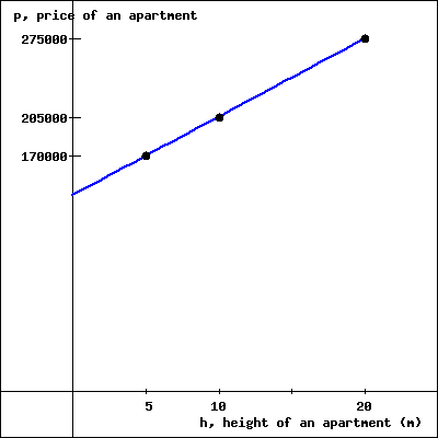
Find a formula for the linear equation graphed below. You can enlarge the graph by clicking on it.
(click on the image to enlarge)
\(p = f(h) =\)
Answer.
\(7000h+135000\)
Solution.
SOLUTION\(p = b + mh\)
\begin{equation*} m = \frac{ \Delta p}{\Delta h} = \frac{275000 - 205000}{20 - 10} = 7000 \end{equation*}
\(b\text{,}\)\(p\)
\begin{equation*} 205000 = b + 7000 \cdot 10 \end{equation*}
\(135000 = b\text{.}\)\(p = f(h) = 135000 + 7000 h\text{.}\)

2.

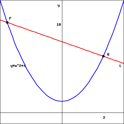
Find the equation for the line \(L\) (graphed in red) in the figure below. Note the \(x\)-coordinate of the point \(Q\) is 2, \(y\)-coordinate of the point \(P\) is 10, and the parabola (graphed in blue) has equation \(y = x^2 + 4\text{.}\)
(click on the image to enlarge)
\(y =\)
Answer.
\(\frac{2}{-\sqrt{6}-2}\mathopen{}\left(x-2\right)+8\)
Solution.
SOLUTION\(P\)\(Q\)\(y = x^2 +4\)\(Q\)\(x\)\(y = 2^2 + 4 = 8\text{.}\)\(P\)\(y\)
\begin{equation*} \begin{aligned} 10 \amp = x^2 + 4, \\ x^2 \amp = 6, \quad\mbox{so} \\ x \amp = \pm \sqrt{6}. \end{aligned} \end{equation*}
\(x = - \sqrt{6}\)\(x \lt 0\text{.}\)\(P\)\(Q\text{,}\)
\begin{equation*} m = \frac{\Delta y}{\Delta x} = \frac{10-8}{- \sqrt{6} - 2} = \frac{2}{- \sqrt{6} - 2}. \end{equation*}
\(y = 8\)\(x = 2\text{,}\)
\begin{equation*} y = \left( \frac{2}{- \sqrt{6} - 2} \right) (x-2) + 8. \end{equation*}

5.

Find the zeros, if any, of the function \(y = 8-4\mathopen{}\left(x-3\right)^{2}\text{.}\)
Enter your answer as a comma separated list. If no zeros exist, enter NONE.
The zeros are \(x =\)
Answer.
\(4.41421, 1.58579\)
Solution.
SOLUTION
We can solve the equation \(8-4\mathopen{}\left(x-3\right)^{2} = 0\) algebraically.
\begin{equation*} \begin{array}{rcl} 8-4\mathopen{}\left(x-3\right)^{2} \amp = \amp 0 \\ -4(x - 3)^2 \amp = \amp -8 \\ (x - 3)^2 \amp = \amp + 2 \\ x - 3 \amp = \amp \pm \sqrt{ + 2} \\ x \amp = \amp + 3 \pm \sqrt{ + 2}. \end{array} \end{equation*}

6.

Find the zero(s) (if any) of the function \(y = x^2 - 9 x + 20\)
Enter your answer as a comma separated list. If no real zeros exist, enter NONE.
The zero(s) is/are \(x =\)
Answer.
\(4, 5\)
Solution.
SOLUTION\(0 = x^2 - 9 x + 20\)\(y = (x - 4)(x - 5)\text{.}\)\(x= 4\)\(x= 5\text{.}\)