So far, you have learned about the different types of algebraic functions. In this section we discuss functions that are NOT algebraic functions. Instead, they are pieced together by parts of algebraic functions.
A piecewise-defined function is is a function that is defined in multiple pieces, with different formulas or rules for different parts of its domain. The sign function defined below is a natural first example in light of our recent work with sign diagrams.
The notation in (1.59) is our way of presenting the different rules that apply to the different subsets of the domain. In general if the domain of our piecewise-defined functionis broken up into subsets \(D_1, D_2,\dots,\text{,}\) then the notation
is understood as defining \(f\) to be the function that follows the rule (or formula) \(f_1\) on the ``domain piece" \(D_1\text{,}\)\(f_2\) on the ``domain piece" \(D_2\text{,}\) etc.. In the case of the sign function, the three different rules are particular simple: namely, the function outputs 1, 0, or -1 depending on whether the input is positive, zero, or negative.
Once you get used to the notation, you will see that working with piecewise-defined functions is done much the same as usual. However, because the a piecewise function is defined in cases, our computations involving these functions naturally break up into cases (or parts).
For example, when graphing the \(\sgn\) function, we effectively make three separate graphs over the separate pieces of the domain: we graph the constant function \(f(x)=1\) on \((0,\infty)\text{,}\) we graph the function \(f_2(x)=-1\) on \((-\infty, 0)\text{,}\) and we add the single point \((0,0)\) to complete the graph.
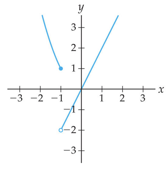
To graph \(f\) we graph the function \(g(x)=x^2\) on the domain \((-\infty, -1]\) and the function \(h(x)=2x\) on the domain \((-1,\infty)\text{.}\) Note that we must be careful about the value of \(f\) at the cutoff input \(x=-1\text{.}\) Since this value is included in the first case of the definition, we have \(f(-1)=(-1)^2=1\text{,}\) corresponding to the point \(P=(-1,1)\) on the graph below.
SubsectionAn Application of Piecewise-defined Functions
Piecewise-defined functions are useful for many real-word problems where the relationship between the quantities involved are different on different time-frames. For example, a person’s salary changes when they get a raise, which changes the amount that they earn each year.
Suppose that in your first job after graduating from college you make $36,000 a year before taxes. After four years you get a raise of $2,500. Two years after that you change jobs and go to work for a company that pays you $49,000 a year.
We can construct a piecewise-defined function that describes your pretax income in the year that is \(t\) years after you graduate from college as follows. Note that this is just the function that describes your income rate per year at a time \(t\) (the units are dollars per year).
\begin{equation*}
\text{ income } (t) = \begin{cases}36000,\amp \text{ if } 0\leq t\lt 4\\ 38500,\amp \text{ if } 4\leq t\lt 6\\ 49000,\amp \text{ if } t\geq6 \end{cases}
\end{equation*}
What may be more interesting is to describe that amount that you will have earned\(t\) years after graduating from college. During the first four years, you make $36,000 per year, and so the amount that you earn after \(t\) years is \(36000t\text{.}\) After four years, you have already earned $\(36,000\cdot 4 = 144,000\text{.}\) Then for the next two years, you earn $38,500 per year, so your additional income for \(4\leq t\lt 6\) is given by \(38500(t-4)\) (because we have to measure in years since\(t=4\)). Thus overall for \(4\leq t\lt 6\text{,}\) you have earned \(144000+38500(t-4)\) by time \(t\text{.}\) Lastly, after 6 years you have earned $\(36,000\cdot 4+38,500\cdot2 = 221,000\text{,}\) and for each additional year you earn $49,000, so by time \(t\) you have earned \(21000+4900(t-6)\) when \(t\geq 6\text{.}\)
If you continue at that pay rate, how long will it have taken you to earn a million dollars? Well, we know we did not make that much by \(t=6\text{,}\) so we use the equation for \(t\geq 6\) and solve for \(t\text{:}\)
How much will you have earned five years after graduating, according to the model described in Example Example 1.10.5? What is your salary in that year?
For the rest of the section we will focus on one specific example of a piecewise-defined function that plays an essential role in calculus: the absolute value function\(f(x)=\abs{x}\text{.}\) What makes this function so valuable to us, is that it introduces a quantitative notion of distance to points on the real number line. Indeed, our first definition of the absolute value will be expressed entirely in these geometric terms.
Given a real number \(x\in \R\) we define its absolute value to be the its distance from 0 on the number line. In more detail, \(\abs{x}\) is the length of the line segment between \(0\) and \(x\text{.}\)
The diagram in Figure 1.10.9 illustrates how we compute \(\abs{x}\) using our geometric definition in terms of distance. From the indicated distances there, we see that
The first piece of information is given by the sign of \(x\text{:}\) that is, \(x\) lies to the left of \(0\) if and only if \(x< 0\text{,}\) and to the right if and only if \(x> 0\text{.}\) The second piece of information is given by the absolute value \(\abs{x}\text{.}\) In this light, you can think of the absolute value function as ignoring the sign of a number and just returning its distance to zero. This is another explanation of why \(\abs{a}=\abs{-a}\text{.}\)
Remark1.10.10.Large and small, greater than and less than.
The foregoing discussion brings to light some linguistic subtleties surrounding mathematical notions like the \(<\) relation, the \(>\) relation, and the absolute value \(\abs{x}\text{.}\)
Namely, although the two relations \(<\) and \(>\) are translated into English as “less than” and “greater than”, a statement like \(x< y\) is not an indication of the relative size (or magnitude) of \(x\) and \(y\text{,}\) but rather their relative position on the real number line! In this sense, the correct geometric way to think of the statement \(x< y\) is as follows:
\begin{align*}
x< y \amp \iff x \text{ lies to the left of } y \text{ on the number line} \\
\amp \iff y \text{ lies to the right of } y \text{ on the number line} \text{.}
\end{align*}
By contrast, the size of a number \(x\) is measured by its absolute value \(\abs{x}\text{.}\) Moreover, to say one number is smaller or larger than another is to say its absolute value is less than or greater than the other number’s absolute value: i.e., we have
\begin{align*}
\abs{x}< \abs{y} \amp \iff x \text{ is smaller than } y\\
\amp \iff y \text{ is larger than } x\text{.}
\end{align*}
As a result, the sign of a number has nothing to do with its size! To illustrate this, note that the three sequences of numbers below are all examples where the terms are getting arbitrarily large:
In more detail we say that the first is a sequence of positive numbers that get arbitrarily large, the second a sequence of negative numbers that get arbitrarily large and negative, and the third a sequence of numbers of alternating sign that get arbitrarily large.
Our geometric definition of the absolute value function in terms of distance will be very important for conceptualizing calculus notions like limits, continuity, and derivatives. However, for computaitonal purposes it is convenient to have a more algebraic definition of the absolute value. Here the notion of a piecewise-defined function comes to our aid.
This example illustrates how, despite the \(-x\) appearing in the formula for the second case of Definition 1.10.11, the output of the absolute value function is always nonnegative.
As the last example illustrates, despite the \(-x\) formula appearing in the second case of the piecewise definition of \(\abs{x}\text{,}\) the output is always nonnegative. This is because the second case only applies if the the input \(x\) is itself negative, in which case the output \(-x\) is positive!
With two separate definitions of the absolute value in play, the question naturally arises whether they agree! The last example gives evidence to the fact that they do. Here is how to see this more generally. For any real number \(x\text{,}\) we can write \(x=a\) or \(x=-a\text{,}\) where \(a\) is a nonnegative number. Since Definition 1.10.11 defines \(\abs{x}\) in cases, it is natural to look at the two cases \(x=a\) and \(x-a\) separately.
If \(x=a\) for some nonnegative number \(a\text{,}\) then it lies a distance of \(a\) to the right of \(0\text{,}\) and hence we should have \(\abs{x}=a\) according to Definition 1.10.8. Using Definition 1.10.11, we have
The other case is similar. Suppose \(x=-a\) for some nonnegative number \(a\text{.}\) In this case \(x\) lies a distance of \(a\) to the left of \(0\text{,}\) and hence has absolute value \(\abs{x}=a\) according to Definition 1.10.8. We get the same result using Definition 1.10.11, since
This arguing by case can be seen at work in the proof of the next result, which among other things, shows that the absolute value function is in fact an algebraic function!
First observe that identity (1.61) implies that \(f(x)=\abs{x}\) is algebraic as it can written as a composition of two power functions. We will use Definition 1.10.11 to prove the identity, and thus argue the two cases \(x\geq 0\) and \(x< 0\) separately.
Assume \(x\geq 0\text{.}\) First observe that by definition \(\sqrt{x^2}\) is the unique nonnegative square-root of \(x^2\text{.}\) Since \(x\) is clearly a square-root of \(x^2\text{,}\) and since \(x\geq 0\text{,}\) we have
It is a very common error, among students and instructors alike, to omit the absolute value in the identity (1.61) and erroneously simplify the expression \(\sqrt{x^2}\) to \(x\text{.}\) To see why this is invalid, it is enough to consider the example \(x=-1\text{:}\)
The example also illustrates what exactly the issue is here: the principal square root function \(\sqrt{\underline{\phantom{xx}}}\) always picks out the nonnegative square root of its input. In particular, its output can never be negative. This alone guarantees that \(\sqrt{(-1)^2}\ne -1\text{.}\)
One explanation for the prevalence of this error is that in many cases it is tacitly assumed that \(x\) is nonnegative, in which case the identity holds without the absolute value since \(\sqrt{x^2}=\abs{x}=x\) for all \(x\geq 0\text{.}\)
The moral of the story is that the validity of a given identity depends very much on the precise scope of its application. Put another way, the quantifier expression “for all \(x\) satisfying...” plays a very important role in the statement of the identity. Sometimes, when stating an identity, we will include this quantifier expression for clarity. For example, here are two correct identities involving a similar equality, but different scopes of application:
\begin{align*}
\sqrt{x^2} \amp =x \text{ for all } x\geq 0\\
\sqrt{x^2} \amp =\abs{x} \text{ for all } x\in \R\text{.}
\end{align*}
The identity \(\abs{x}=\sqrt{x^2}\) allows us to derive many useful properties of the absolute value function from those of the principal square-root function. Furthermore, knowing now that \(f(x)=\abs{x}\text{,}\) we can make use of Theorem 1.8.11 and Procedure 1.8.12 to deterimine solutions to inequalities involving the absolute value. We include these results here in one compendium result. We will spare you the details of a proof, but invite you to think on your own about how you would proves these facts.
In plain English: the absolute value of a product is the product of the absolute values, and the absolute value of a quotient is the quotient of the absolute values.
\begin{align}
\abs{x}= a \amp \iff x=a \text{ or } x=-a\tag{1.64}\\
\abs{x}< a\amp \iff -a< x < a \tag{1.65}\\
\abs{x}> a \amp \iff x> a \text{ or } x< -a \text{.}\tag{1.66}
\end{align}
Here the last line follows from a sign analysis of \(f(x)=(x-3)(x+1)\) (or alternatively, by constructing a sign diagram) and the fact that \((x-1)^2+2\geq 2\) for all \(x\text{,}\) and hence never satisfies \((x-1)^2+2< 0\text{.}\) We conclude that the solution set is \((-\infty, -1)\cup (3,\infty)\text{.}\)
The notion of distance \(d(a,b)=\abs{a-b}=\abs{b-a}\) between points on the real line will be used extensively in our development of calculus. This in turn is why a solid understanding of the absolute value function is so important. We content ourselves with a few short comments.
Note that our definition (1.67) generalizes the distance to 0 formula, since for any \(x\in \R\) we have
The fact that \(d(a,b)\) is the length of the line segment between \(a\) and \(b\) can be shown to follow from Definition 1.10.8 using a nice “shift argument”. By way of illustration, consider \(a=-3\) and \(b=7\text{.}\) Shifting these points to the right by three units yields new points \(a'=0\) and \(b'=10\text{.}\) Shifting the two points this way does not change the distance between them: i.e., \(d(a,b)=d(a',b')\text{.}\) It follows that
Fix a point \(a\) on the real line. The closeness or farness of a variable point \(x\) to \(a\) is measured by its distance \(d(x,a)=\abs{x-a}\text{.}\) Thus we have
\begin{align*}
x \text{ close to } a \amp \iff \abs{x-a} \text{ is small (i.e. close to zero)}\\
x \text{ far from } a \amp \iff \abs{x-a} \text{ is large}\text{.}
\end{align*}
It remains only to consider the graph of \(f(x)=\abs{x}\text{,}\) and more generally, graphs of functions involving absolute value. Using the piecewise definition of \(f(x)=\abs{x}\text{,}\) we can produce its graph very easily by looking at the two cases \(x\geq 0\) and \(x< 0\) separately. We have
Thus the graph of \(f\) is given by the graph of the line \(y=x\) for all \(x\geq 0\) and the line \(y=-x\) for all \(x< 0\text{.}\) This gives rise to the vee-shaped graph in Figure 1.10.20.
More generally, how do we graph a function of the form \(f(x)=\abs{g(x)}\text{?}\) We can analyze this question using the piecewise definition of absolute value, along with our graphical interpretation of the scaling transformation. By definition, we have
Thus we can obtain the graph of \(f(x)=\abs{g(x)}\) by graphing \(g(x)\) at all \(x\) where \(g(x)\geq 0\text{,}\) and \(-g(x)\) at all \(x\) where \(g(x)< 0\text{.}\) Since the graph of \(-g\) is the result of reflecting the graph of \(g\) over the \(x\)-axis, we see that \(f(x)=\abs{g(x)}\) can be obtained by beginning with the graph of \(g\) and flipping all portions of the graph where \(g< 0\text{.}\) Let’s make this an official procedure for good measure.
The graph of \(f(x)=\abs{g(x)}\) is obtained from the graph of \(g\) by finding all portions of the graph of \(g\) where \(g< 0\) and reflecting these over the \(x\)-axis.
Example1.10.22.Transformed absolute value function.
Consider the function \(f(x)=\abs{2x-1}\text{.}\) We have \(f(x)=\abs{g(x)}\text{,}\) where \(g(x)=2x-1\text{.}\) Since \(g(x)< 0\) if and only if \(x< 1/2\text{,}\) we obtain the graph of \(f\) by flipping the part of the line \(y=2x-1\) that lies below the \(x\)-axis across the \(x\)-axis.
Consider \(f(x)=\abs{x^2-1}=\abs{g(x)}\text{,}\) where \(g(x)=x^2-1\text{.}\) Our usual sign diagram argument shows that \(g(x)< 0\) if and only if \(-1< x< 1\text{.}\) Thus we obtain the graph of \(f\) by flipping the part of the parabola \(g(x)=x^2-1\) lying over the interval \((-1,1)\) across the \(x\)-axis.