Definition 2.16.21 ties the values of \(\cos\theta\) and \(\sin\theta\) intimately to the geometry of the unit circle with defining equation \(x^2+y^2=1\text{.}\) As a result we can easily prove some useful properties about \(\cos\) and \(\sin\text{,}\) and their relationship to one another.
The Pythagorean identity follows almost immediately from the definition of \(\cos\) and \(\sin\text{.}\) Given any angle \(\theta\text{,}\) let \(P=(x,y)\) be the point where the terminal edge of \(\theta\) intersects the unit circle. By definition of the unit circle, \(x\) and \(y\) satisfy \(x^2+y^2=1\text{.}\) By definition of \(\cos\) and \(\sin\text{,}\) on the other hand, we have \(\cos\theta=x\) and \(\sin\theta=y\text{.}\) We conclude that \(\cos^2\theta+\sin^2\theta=1\text{.}\)
For any \(\theta\in \R\text{,}\) the two angles \(\theta\) and \(\theta+2\pi\) are coterminal. As a result, both angles are associated to the same point \(P=(x,y)\text{,}\) following the recipe of Definition 2.16.21. We conclude that
Given any \(\theta\in \R\text{,}\) we have \(\cos\theta=x\) and \(\sin\theta=y\text{,}\) where \(P=(x,y)\) is a certain point on the unit circle. Since by definition of the unit circle these coordinates satisfy \(x^2+y^2=1\text{,}\) it is easy to see that we must have \(\abs{x}\leq 1\) and \(\abs{y}\leq 1\text{,}\) or equivalently,
We conclude that \(-1\leq \cos\theta\leq 1\) and \(-1\leq \sin\theta\leq 1\) for all \(\theta\in \R\text{,}\) and thus \(\range \cos\subseteq [-1,1]\) and \(\range \sin\subseteq [-1,1]\text{.}\)
We now show that in fact we have \(\range \cos=\range\sin=[-1,1]\text{.}\) Given any \(a\in [-1,1]\text{,}\) since \(\abs{a}\leq 1\text{,}\)we may define \(b=\sqrt{1-a^2}\text{.}\) Since \(b^2=1-a^2\text{,}\) it is easy to see that \(b\in [0,1]\) and that
Thus \(P=(a,b)\) is a point on the unit circle. Letting \(\theta\) be the central angle in standard position subtended by the arc from \((1,0)\) to \(P\text{,}\) we see that \(\cos\theta=a\text{.}\) This proves \(\range \cos=[-1,1]\text{.}\) A similar argument shows that \(\range \sin=[-1,1]\text{.}\)
Adding a suitable multiple of \(2\pi\) and using periodicity, we may assume that \(\theta\in [0,2\pi]\) and \(-\theta\in [-2\pi,0]\text{.}\) Let \(P=(x,y)\) be the point where the terminal edge of \(\theta\) intersects the unit circe, and let \(P'=(x',y')\) be the point where the terminal edge of \(-\theta\) intersects the intersection of the unit circle. The oriented arc associated to \(\theta\) starts from \((1,0)\text{,}\) moves counterclockwise and ends at \(P\text{;}\) the oriented arc associated to \(-\theta\) traverses the same length of the circle (since \(\abs{\theta}=\abs{-\theta}\)) starting from \((1,0)\text{,}\) but in the clockwise direction. It follows that the latter arc is just the reflection of the former arc across the \(x\)-axis. As a result we have \(x'=x\) and \(y'=-y\text{.}\) We conclude that
Given any \(\theta\in \R\text{,}\) adding a suitable multiple of \(2\pi\) and using periodicity, we may assume that \(\theta\in [0,2\pi]\text{.}\) If \(\theta\in [\pi,2\pi]\text{,}\) then \(-\theta\) is coterminal to an angle in \([0,\pi]\text{.}\) Since \(\cos(-\theta)=-\cos\theta\) and \(\sin(\pi-(-\theta))=\sin(\pi+\theta)=-\sin\theta\text{,}\) we see that \(\cos\theta=\sin(\pi/2-\theta)\) if and only if \(\cos(-\theta)=\sin(\pi/2-(-\theta))\text{.}\) Thus we may assume that \(\theta\in [0,\pi]\text{.}\) Since, furthermore, the result is easily verified for \(\theta=0\) and \(\theta=\pi\text{,}\) we assume that \(\theta\in (0,\pi)\text{.}\) Let \(P=(x,y)\) be the point where the terminal edge of \(\theta\) intersects the unit circle, and let \(T\) be the corresponding reference triangle with vertices \((0,0)\text{,}\)\(P\text{,}\) and \((x,0)\) obtained by dropping the perpendicular from \(P\) to the \(x\)-axis.
Consider the the case where \(\theta\) is acute: i.e., \(\theta\in (0,\pi/2)\text{.}\) In this case the angle of \(T\) at \((0,0)\) is \(\theta\) and the angle of \(T\) at \(P\) is \(\pi/2-\theta\text{,}\) since \(T\) is a right triangle. Using triangular interpretations of \(\cos\) and \(\sin\text{,}\) we conclude that
The case for \(\theta\) obtuse (i.e., \(\theta\in (\pi/2, 2\pi)\)) is similar, with some sign details. The point \(P=(x,y)\) is now in the second quadrant of the plane, which means the \(x\)-coordinate is negative. Now the angle at \((0,0)\) is \(\pi-\theta\text{,}\) and the angle at \(P\) is \(\pi/2-(\pi-\theta)=\theta-\pi/2\text{.}\) The same triangular reasoning as above can be applied, but now we have to be careful about sign: we have \(\sin(\theta-\pi/2)=\abs{x}=-x\) in this case, since \(x\leq 0\text{.}\) Using the oddness of sine, we conclude that \(\sin(\pi/2-\theta)=x\text{,}\) as desired!
The interdependence of \(\cos\) and \(\sin\) articulated in Theorem 2.18.1, allows us in many situations to derive the value of one of the two function \(\cos\) and \(\sin\) from the other, at least up to sign. The next example illustrates this idea.
Example2.18.2.Interdependence of \(cos\) and \(\sin\).
For a fixed but indeterminate angle \(\theta\text{,}\) information about one of the two values \(\cos\theta\) and \(\sin\theta\) is given. If possible, determine the value of the other function; if not, explain why the exact value cannot be determined.
We see that there are two possible values of \(\sin\theta\text{.}\) Without further information, we cannot determine which one applies in the given situation. Indeed, there are two separate points \(P=(-1/3, 2\sqrt{2}/3)\) and \(Q=(-1/3,-2\sqrt{2}/3)\) on the unit circle with \(x\)-coordinates equal to \(-1/3\text{.}\) Letting \(\theta\) be the angle associated to \(P\text{,}\) we have \(\cos\theta=-1/3\) and \(\sin\theta=2\sqrt{2}/3\text{.}\) Similarly, letting \(\theta\) be the angle associated to \(Q\text{,}\) we have \(\cos\theta=-1/3\) and \(\sin\theta=-2\sqrt{2}/3\text{.}\)
Again, we so far only know \(\cos\theta\) up to sign. However, since \(\theta\in [pi/2, 3\pi/2]\text{,}\) the point associated to \(\theta\) is in the second or third quadrant of the plane, where the \(x\)-coordinate is always negative. (See Figure 2.17.5.) We conclude that \(\cos\theta=-\frac{\sqrt{21}}{5}\text{.}\)
The properties of \(\cos\) and \(\sin\) spelled out in Theorem 2.18.1 are readily interpreted visually in terms of the graphs of these two functions. For example, the fact that \(\range\cos=\range\sin=[-1,1]\) tells us that the \(y\)-coordinates of points on the these graphs always lie between \(-1\) and \(1\text{,}\) and furthermore that every value in that range is the \(y\)-value of some point on the graph. Next, the fact that \(\cos\) and \(\sin\) both have period \(2\pi\) tells us that once we know what the graph looks like over the interval \([0,2\pi]\) (or any interval of length \(2\pi\)), we can produce the rest of the graph by “cutting and pasting”: in more detail, take the graph of the function over \([0,2\pi]\) and simply shift to the right by \(2\pi\) to get the graph over \([2\pi, 4\pi]\text{;}\) similarly, shift to the left by \(2\pi\) to get the graph over \([-2\pi, 0]\text{.}\) Lastly, the even/odd properties of \(\cos\) and \(\sin\) tell us the usual symmetry properties of graphs of even and odd functions. (See Definition 1.6.24 and the discussion that follows it.)
But what exactly does the graph of one these functions look like for \(x\in [0,2\pi]\text{.}\) We can give a fairly precise qualitative description of this by examining what happens to the \(x\)-coordinate of the point \(P_\theta\) associated to the central angle \(\theta\text{,}\) as we let \(\theta\) range from \(0\) to \(2\pi\text{.}\) It is useful to think of this as an animation, where the point \(P_\theta\) associated to \(\theta\) travels all the way around the unit circle as we \(\theta\) increases from \(0\) to \(2\pi\text{.}\) Focusing just on the \(x\)-coordinate of \(P_\theta\text{,}\) we deduce the following qualitative summary.
As \(\theta\) increases from \(0\) to \(\pi/2\text{,}\) the \(x\)-coordinate of \(P_\theta\) decreases from \(1\) to \(0\text{.}\)
Remembering that \(\cos \theta\) is by definition the \(x\)-coordinate of this point \(P_\theta\text{,}\) our summary above leads pretty directly to the graph of \(\cos\theta\) below. We have enhanced this sketch with some actual plotted points: namely, the point \((\theta, \cos\theta)\text{,}\) for each of the 16 familiar angles from Figure 2.17.13.
A similar description can be obtained for the graph of \(\sin\) by looking at the \(y\)-coordinates of the points \(P_\theta\) as \(\theta\) ranges from \(0\) to \(2\pi\text{.}\) These values begin at \(0\text{,}\) increase to \(1\) as \(\theta\) increases from \(0\) to \(\pi/2\text{,}\) decrease back to \(0\) as \(\theta\) increases from \(\pi/2\) to \(\pi\text{,}\) decrease further to \(-1\) as \(\theta\) increases from \(\pi\) to \(3\pi/2\text{,}\) and finally increase back to \(0\) as \(\theta\) increases from \(3\pi/2\) to \(2\pi\text{.}\) Identifying this changing \(y\)-value of \(P_\theta\) with \(\sin\theta\text{,}\) we obtain the following graph.
Understanding the basic pattern of the changing values of \(\cos\) and \(\sin\) allows us to quickly give a detailed sketch of these functions. Incorporating our shifting and scaling techniques, it is then not difficult to obtain the graphs of more general functions of the form
where \(A,B,k\) are fixed constants. Such functions are called sinusoidal. Here is a summary of these parameters affect the graphs of the functions. We work from the inner most operation (multiplying \(x\) by \(k\)) to the outermost (adding \(B\))
Assume \(k> 0\text{.}\) Scaling the input \(\theta\) by \(k\) shrinks the graph of \(\cos\) horizontally by \(1/k\text{.}\) As a result, the period of the functions \(f(\theta)=\cos k\theta\) and \(g(\theta)=\sin k\theta\) is \(2\pi/k\text{.}\)
Since scaling by \(A\) scales the \(y\)-values of the graph of \(\cos\) or \(\sin\) by a factor of \(A\text{,}\) the functions \(f(\theta)=A\cos k\theta\) and \(g(\theta)=A\sin k\theta\) vary (or oscillate) between \(-A\) and \(A\text{.}\) Accordingly, \(\abs{A}\) is called the amplitude of the the functions \(f\) and \(g\text{.}\) The amplitude measures how much the \(y\)-values vary from midline \(y=0\) of the graph of \(f\) and \(g\text{.}\)
Lastly, the parameter \(B\) shifts the graph vertically by \(B\text{.}\) As a result, the midline of the functions \(f(\theta)=A\cos k\theta+B\) and \(g(\theta)=A\sin k \theta+B\) is shifted from \(y=0\) to \(y=B\text{.}\)
Let \(f(\theta)=A\cos k \theta+B\) and \(g(\theta)=A\sin k\theta+B\text{,}\) where \(A\) and \(k\) are positive constants, and \(B\) is any constant. To produce a graph of \(f\) and/or \(g\text{,}\) proceed as follows.
Determine period.
The period of \(f\) and \(g\) is \(2\pi/k\text{.}\)
The midline of \(f\) and \(g\) is the horizontal line \(y=B\text{.}\) The amplitude of \(f\) and \(g\) is \(\abs{A}=A\text{,}\) which means the \(y\)-values of these functions vary between \(B-A\) and \(B+A\text{.}\) Draw the dotted lines \(y=B-A\text{,}\)\(y=B\text{,}\) and \(y=B+A\) on your coordinate plane. These will help scaffold your graph of \(f\) and \(g\text{,}\) as they indicate the bottom, middle, and top of the graph.
In the given situation, where \(A\) and \(k\) are both positive, the \(y\)-values of these 5 plotted points follow the bottom/middle/top patterns below.
For \(f(\theta)=A\cos k \theta+B\text{,}\) the points follow the “cosine” pattern: top-middle-bottom-middle-top.
Extend the graph horizontally as much as you like by shifting the graph for \(\theta\in [0,2\pi/k]\) to the right and/or left by integer multiples of \(2\pi/k\text{.}\)
We assume \(A\) and \(k\) are positive in Procedure 2.18.5 only for convenience. The case where either one of these parameters is negative can be derived from the positive case by making use of an appropriate reflection: either through the midline \(y=B\) (if \(A\) is negative), or through the \(y\)-axis (if \(k\) is negative).
In the case where \(A\) is negative, the cosine and sine patterns described in Step 3 of Procedure 2.18.5 are flipped about the midline. In more detail, if \(A<0 \text{,}\) then the 5 plotted points of \(f\) follow the “negative cosine pattern” (bottom-middle-top-middle-bottom), and the 5 plotted points of \(g\) follow the “negative sine pattern” (middle-bottom-middle-top-middle).
In this case we have \(A=3\text{,}\)\(k=1/2\text{,}\) and \(B=-1\text{.}\) It follows that the period of \(f\) is \(2\pi/(1/2)=4\pi\text{,}\) the midline is \(y=-1\text{,}\) and the \(y\)-values of the graph of \(f\) oscillate between \(y=-1-3=-4\) and \(y=-1+3=2\text{.}\)
We divide the period interval \([0,4\pi]\) into \(4\) equal subintervals and plot points with inputs \(0,\pi, 2\pi, 3\pi, 4\pi\text{.}\) Since \(f\) is defined in terms of \(\cos\text{,}\) these plotted points follow the top-middle-bottom-middle-top “cosine pattern”. Putting this all together, we obtain the graph in Figure 2.18.8.
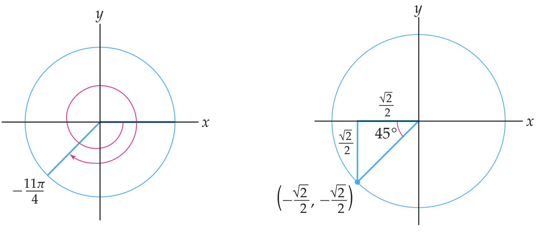
Sketch the angle \(-\frac{11\pi}{4}\) in standard position, and then use the unit circle to find the values of all six trigonometric functions of that angle.
Since \(2\pi\) radians is one full revolution around the unit circle, the angle \(-\frac{11\pi}{4}\) opens up in the clockwise direction for one full revolution and then an additional three-quarters of the bottom half of the unit circle, as shown at the left:
In the right-hand picture above, we see a 45-45-90 reference triangle with the labeled side lengths of \(\sqrt{2}/2\text{.}\) Because the angle terminates in Quadrant III, both coordinates of the point on the unit circle are negative. By the unit-circle definitions of sine and cosine,
Graphs of these additional trigonometric functions are provided in Figure 2.18.11. The general shape and distinguishing properties of these graphs, including their vertical asymptotes, are easily deduced from our knowledge of the behavior and graphs of \(\cos\) and \(\sin\text{.}\) When needed, explicitly plotted points can be added to these graphs by evaluating functions at any of the 16 familiar angles from Figure 2.17.13 lying in their domain.
From the graphs we can immediately deduce properties of the range of the remaining trigonometric functions. For example, we see that the \(y\)-coordinates of points on the graphs of \(\tan\) and \(\cot\) span all possible real values, telling us that \(\range \tan=\range \cot=\R\text{.}\) By contrast, the \(y\)-coordinates of points on the graphs of \(\sec\theta\) and \(\csc\theta\) are restricted to the intervals \((-\infty, -1]\) and \([1,\infty)\text{,}\) and include all possible values in those intervals. Strictly speaking, to rigorously justify these claims we need to use an intermediate value argument; and for this we need to know that these functions are continuous. We will establish this fact soon enough, but will make our range observations official in the meantime.
To better conceptualize the behavior of \(\tan\theta\) as \(\theta\) varies, the following slope interpretation can be helpful. Given \(\theta\in \R\text{,}\) let \(P_\theta=(x,y)\) be the intersection of the terminal edge of the central angle \(\theta\) with the unit circle, as usual, let \(\ell_\theta\) be the line passing through the origin and \(P_\theta\text{.}\) As illustrated in Figure 2.18.14, the slope \(m_\theta\) of \(\ell_\theta\) is given by
As we let \(\theta\) increase from \(\theta=0\text{,}\) the line \(\ell_\theta\) rotates counterclockwise about the origin, and as it does so its slope \(m_\theta=\tan\theta\) varies. This allows us to tell the following story about \(\tan\theta\) as \(\theta\) varies through various intervals of the real line.
As \(\theta\) increases from \(0\) and approaches \(\pi/2\text{,}\) the slope \(m_\theta\) of the line \(\ell_\theta\) starts off at \(0\text{,}\) gets increasingly positive, and approaches \(\infty\) as \(\theta\) approaches \(\pi/2\text{.}\) Thus \(\tan \theta\) begins has starting value \(0=\tan 0\text{,}\) and increases without bound as \(\theta\) approaches \(\pi/2\text{.}\)
Similarly, as \(\theta\) decreases from \(0\) and approaches \(- \pi/2\text{,}\) the slope of the line \(\ell_\theta\) starts off at \(0\text{,}\) gets increasingly negative, and approaches \(-\infty\) as \(\theta\) approaches \(-\pi/2\text{.}\) This means as we decrease \(\theta\) from \(0\text{,}\)\(\tan\theta\) has starting value \(0=\tan 0\) and decreases without bound as \(\theta\) approaches \(-\pi/2\text{.}\)
The fact that \(\tan\theta\) is undefined at \(\theta=\pm \pi/2\) corresponds to the fact that the line \(\ell_\theta\) is vertical at these angles, and thus has undefined slope.
We end this section with two simple geometric applications of the trigonometric functions. The first takes us out of the unit cirle \(x^2+y^2=1\) and uses the trigonometric functions to determine coordinates of points on a circle \(x^2+y^2=r^2\) of arbitrary radius \(r\text{.}\)
Let \(r\in (0,\infty)\text{,}\) and let \(C_r\) be the circle \(x^2+y^2=r^2\) of radius \(r\text{.}\) Given \(\theta\in \R\text{,}\) let \(P_{r,\theta}=(x,y)\) be the intersection of the terminal edge of the standard central angle \(\theta\) with the circle \(C_r\text{,}\) as depicted in Figure 2.18.16. We have
\begin{align}
x \amp =r\cos\theta \amp y\amp=r\sin\theta\tag{2.84}
\end{align}
This slight generalization of the definitions of the trigonometric functions in terms of the unit circle, is a consequence of the law of similar triangles. As indicated in Figure 2.18.17, we simply relate the reference triangle associated to \(P_{r,\theta}\) to the reference triangle for the point \(P_\theta\) where the terminal edge of the angle \(\theta\) intersects the unit circle.
Lastly, we can remove the circles altogether from the context and focus solely on reference triangles. The result is the following classic right-triangle formulation of trigonometric values, often summarized as “SohCahToa”, which itself is a mnemonic for the following statements:
Let \(\theta\) be an acute angle of a right triangle, let \(\text{adj}\) and \(\text{opp}\) denote the lengths of the sides adjacent and opposite to \(\theta\text{,}\) and let \(\text{hyp}\) denote the length of the hypotenuse of the triangle. We have