As we have seen over the last few sections, in order to determine when a function is positive and negative, find the domain of a function involving an even root, and rewrite an absolute value, we will need to be able to work with inequalities. We will need to solve inequalities in order to explore functions in general and answer many interesting questions, and so we summarize the relevant rules and develop the necessary techniques for solving inequalities. Let’s begin by defining what we mean by an "inequality."
An inequality consists of two mathematical expressions related by a greater-than \(>\text{,}\) less-than \(<\text{,}\) greater-than-or-equal-to \(\geq\text{,}\) or less-than-or-equal-to \(\leq\) sign. The solution set of an inequality is the set of all values that make the inequality true. Wheres the solution set of an equation often consists of a finite number of points, the solution set of an inequality is often an interval of real numbers, or unions of intervals.
That is we isolated the \(x\) term by adding \(1\) to both sides of the inequality. The reason why this step is valid is that if \(x< y\text{,}\) then \(x+a< y+a\) for any \(a\in \R\text{:}\) i.e., adding a constant to two numbers preserves the inequality relation between them.
What about multiplying both sides of an equality by a nonzero constant? Is it true that if \(x < y\text{,}\) then \(ax< ay\) for any nonzero \(a\text{?}\) No! Consider the following example: \(1< 2\text{,}\) but \((-2)1=-2\not < -4=(-2)2\text{.}\) We have (re)discovered the first nuance about solving inequalities: multiplying numbers by nonzero constants doesn’t necessarily preserve their inequality relation: in fact, if the constant is negative, the relation is reversed! Below we make official this observation, along with some other elementary inequality rules.
The statements in Theorem 1.8.1 remain true if we place \(<\) with \(\leq\text{.}\) Why? The relation \(\leq\) means less than or equal to. Since the statements above are true with respect to the relation \(<\) (the content of the theorem) and to the relation \(=\text{,}\) it follows logically that they are true with respect to the relation \(\leq\text{.}\)
The English phrases “less than” and “greater than” unfortunately obscure somewhat the meaning of the relations \(<\) and \(>\text{.}\) For example, we are tempted to translate the statement \(x< y\) as “\(x\) is smaller than \(y\)”. But this is not what the \(x< y\) means. Indeed, we have \(-100< 1\text{,}\) and yet \(-100\) is not smaller than \(1\text{.}\) The correct way of understanding \(x< y\) is as a statement about the relative position of \(x\) and \(y\) on the number line. That is, we have
\begin{align*}
x< y \amp \iff x \text{ is to the left of } y \text{ on the number line}\\
x> y \amp \iff x \text{ is to the right of } y \text{ on the number line}\text{.}
\end{align*}
Equipped with the inequality rules of Theorem 1.8.1, we are able to solve elementary inequalities in much the same way we do equalities, but taking due care when multiplying by negative constants or taking reciprocals.
Clearly, we want to use the reciprocal rule here, but we need to be careful since to do so, the signs of both sides of the inequality have to agree! We handle this by separately treating the cases where \(5/(x+1)\) is negative and positive.
Note that \(5/(x+1)< 0\) if and only if \(x+1< 0\) if and only if \(x< -1\text{.}\) In this case we certainly have \(5/(x+1)\leq 8\text{.}\) Thus the interval \((-\infty, -1)\) is part of our solution.
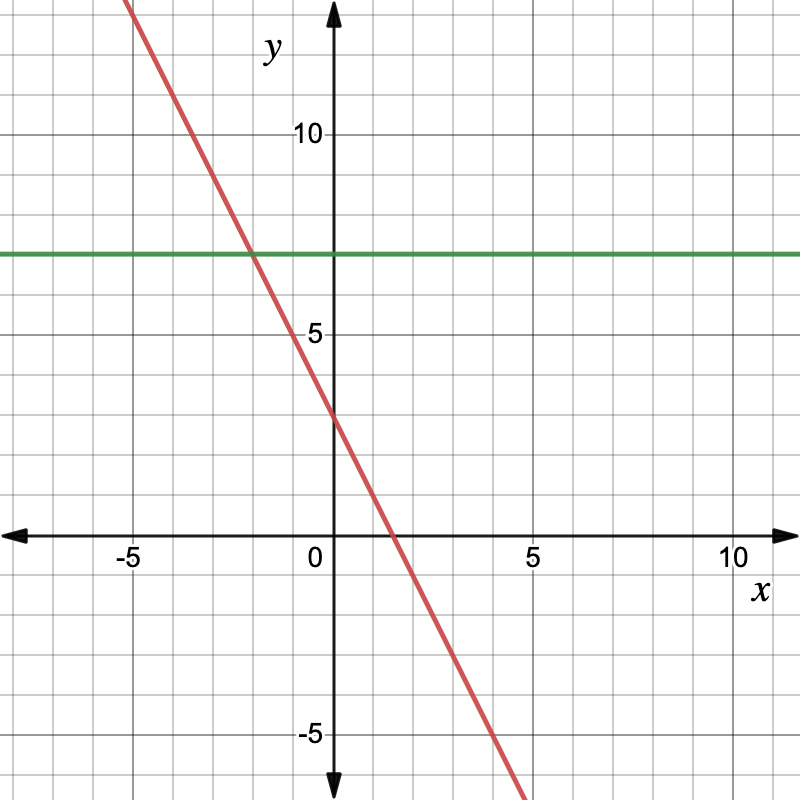
You can check our solution to \(3-2x> 7\) by graphing \(y=3-2x\) (in red) and \(y=7\) (in green), as shown in Figure 1.8.6. The values of \(x\) for which the line described by \(3-2x\) has \(y\)-coordinate greater than \(7\) are those to the left of \(x=-2\text{.}\)
Our solution to the second inequality of Example 1.8.4 illustrates how careful consideration of the signs (positive/negative) involved in an inequality can make the solution even to an elementary looking inequality somewhat involved. The “sign diagram” technique developed later in this section will make these issues much easier to deal with.
Theorem 1.8.1 allows us to solve a linear inequality \(ax+b< c\) almost exactly as we would the corresponding linear equality \(ax+b=c\text{;}\) we just need to be careful about the sign when multiplying both sides by \(1/a\text{.}\) With anything more complicated, however, solving inequalities becomes much more subtle.
Consider the quadratic inequality \(x^2-x< 0\text{.}\) Since adding any constant to both sides preserves the inequality, we can add \(x\) to both sides to conclude
\begin{equation*}
x^2< x\text{.}
\end{equation*}
We might be tempted to multiply both sides of the equation by \(1/x\) (we can exclude \(x=0\text{,}\) since the inequality clearly doesn’t hold for this choice), however we need to remember that depending on whether \(x\) is negative or positive, the inequality might flip. This leads to two separate cases.
Now use the fact that a product of two numbers is negative if and only if the two numbers have different signs:
\begin{align*}
x(x-1) \amp < 0\\
(x< 0 \text{ and } x-1> 0) \amp \text{ or } (x> 0 \text{ and } x-1< 0) \\
(x< 0 \text{ and } x> 1) \amp \text{ or } (x> 0 \text{ and } x< 1) \\
0 \amp < x < 1\text{.}
\end{align*}
Note that the left side of our “or” statement was eventually discarded since there is no number \(x\) satisfying \(x< 0\) and \(x> 1\text{.}\) In all we conclude that the set of solutions to the inequality is the interval \((0,1)\text{.}\)
Let \(a\) and \(b\) be nonzero real numbers. We have \(ab> 0\) if and only if \(a\) and \(b\) have the same sign, and \(ab< 0\) if and only if \(a\) and \(b\) have opposite signs. In other words:
\begin{align*}
ab> 0 \amp \iff a,b> 0 \text{ or } a,b< 0\\
ab< 0 \amp \iff a< 0< b \text{ or } b< 0< a\text{.}
\end{align*}
A similar approach can be used for a more general quadratic inequality \(ax^2+bx+c< d\text{:}\) namely, first make the right side of the inequality 0 (\(ax^2+bx+(c-d)< 0\)); then try to factor the left side (\(a(x-c_1)(x-c_2)< 0\)); then treat the different cases coming from Theorem 1.8.8. However, we are interested in one technique that works not only for quadratic inequalities, but also inequalities involving any algebraic function. This leads us to what we call a sign diagram technique.
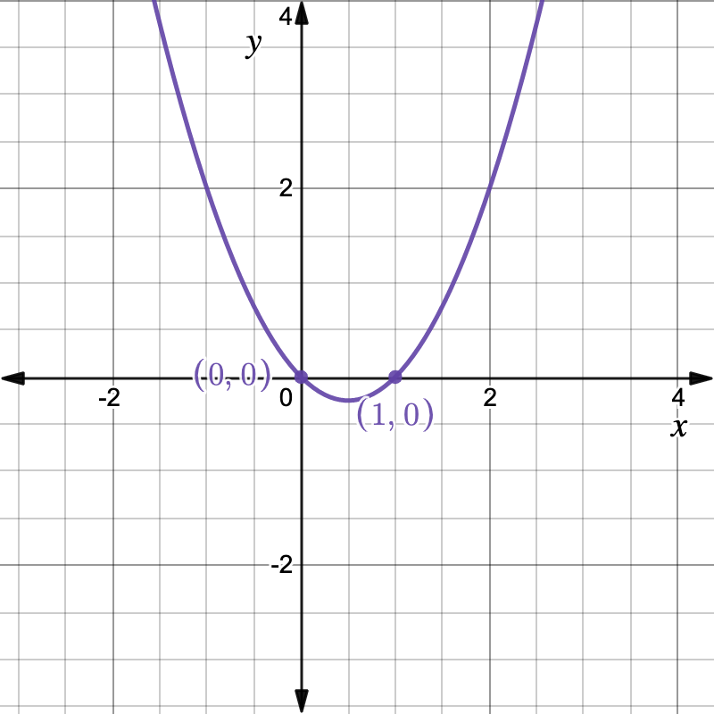
Consider again the inequality \(x^2-x< 0\text{.}\) We can interpret this as a statement about the function \(f(x)=x^2-x\text{:}\) namely, the set of solutions to the inequality is precisely the set of \(x\) where \(f\) is negative. This set is easily visualized by a graph of \(f\text{.}\)
The graph confirms that \(f(x)=x^2-x < 0\) if and only if \(0< x< 1\text{,}\) just as we had deduced above. It also brings to light another property that will be useful for solving inequalities: the sign of the function does not change until we reach a zero. In the example above, we have \(f> 0\) on the entire interval \((-\infty, 0)\text{,}\)\(f< 0\) on \((0,1)\text{,}\) and \(f> 0\) on \((1,\infty)\text{.}\) This is elegantly summarized by the sign diagram of \(f\) below.
As it turns out, this constancy of sign exhibited by \(f(x)=x^2-x\) is enjoyed not just by all quadratic functions, but indeed by all algebraic functions. The property seems intuitively true: a function shouldn’t be able to switch from positive to negative, or vice versa, without crossing the \(x\)-axis. However, to prove this property rigorously, we need some help from calculus: namely, the notion of a continuous function, as well as the intermediate value property that continuous functions enjoy. We will get to these in due time, at which point we will re-visit the discussion here. For now, we will take on faith this property of sign, that we articulate in the theorem below.
Theorem1.8.11.Constancy of sign: algebraic functions.
Let \(f\) be an algebraic function. If \(I\) is an interval containing no zeros of \(f\) and no points where \(f\) is undefined, then \(f\) is either always positive or always negative on \(I\text{.}\)
Theorem 1.8.11 is the theoretical underpinning of the following procedure for solving inequalities. Although the procedure is stated for inequalities of the form \(f(x)< 0\text{,}\)
Identify the sign of \(f\) on the resulting open intervals that have the points in Step 2 as endpoints. This can be done by evaluating \(f\) at a test point in each of these intervals, or by using elementary inequality properties.
The rational function \(f(x)=(-8x-3)/(x+1)=-(8x+3)/(x+1)\) is undefined at \(x=-1\) and has a zero at \(x=-3/8\text{.}\) Thus we begin with the number line diagram
Next we identify the sign of \(f\) on the three intervals \((-\infty, -1)\text{,}\)\((-1,-3/8)\text{,}\)\((-3.8,\infty)\text{.}\) We can do this by using the following test points:
From the constancy of sign theorem, we conclude that \(f< 0\) on \((-\infty, -1)\) and \((-3/8, \infty)\) and \(f> 0\) on \((-1, -3/8)\text{.}\) This is summarized in the following sign diagram for \(f\text{.}\)
Since furthermore, \(f(x)=0\) at \(x=-3/8\text{,}\) we conclude that the set of solutions to \(f(x)\leq 0\text{,}\) and hence to our original inequality (1.57) is \((-\infty, -1)\cup [-3/8, \infty)\text{.}\)
We conclude that the set of solutions to \(f(x)> 0\text{,}\) and hence also \(x^2> a\text{,}\) is \((-\infty, \sqrt{a})\cup (\sqrt{a},\infty)\text{.}\)