Estimating area

Section 1.2 Estimating area

By way of motivation of what will be the definition of the integral, we consider the computational problem of computing the area of a region defined by the graph of a function.

Interactive example 1.2.1. Estimating area.

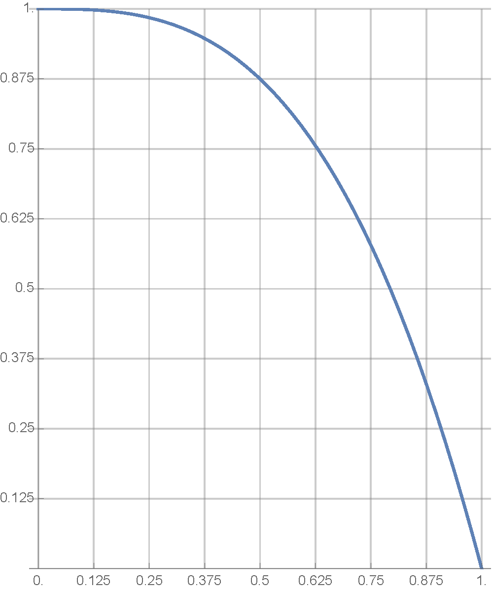
Let \(\mathcal{R}\) be the set of points lying between the graph of \(f(x)=1-x^3\) and the \(x\)-axis from \(x=0\) to \(x=1\text{:}\) that is,

\begin{equation*} \mathcal{R}=\{(x,y)\colon 0\leq x\leq 1, 0\leq y\leq f(x) \}\text{.} \end{equation*}

We will estimate the area of this region by approximating the region itself with a collection of blocks of equal width, whose heights are determined by the \(y\)-values of points on the graph of \(f\) through some means. The GeoGebra interactive below helps illustrate the technique.

Figure 1.2.1. GeoGebra: Estimating area with rectangular blocks ¹

Procedure 1.2.2. Estimating area.

Let \(f\) be a nonnegative function defined on the interval \([a,b]\text{,}\) and let \(\mathcal{C}\) be the graph of \(f\) from \(x=a\) to \(x=b\text{.}\) To estimate the area between \(\mathcal{C}\) and the \(x\)-axis proceed as follows:

Divide \([a,b]\) into \(n\) equal subintervals, each of width \(\Delta x=(b-a)/n\text{.}\)
For each subinterval pick a sample input \(x^*\) in that interval and build the rectangle whose base is the subinterval and whose sample height is given by \(h=f(x^*)\text{.}\) The area of this block is

\begin{equation} A=\underset{\text{ height } }{\underbrace{f(x^*)}}\,\underset{\text{ width } }{\underbrace{\Delta x}}\text{.}\tag{1.2.1} \end{equation}
Sum together the areas of the \(n\) blocks constructed in Step 2.

Depending on how the sample inputs \(x^*\) are chosen in each subinterval, we get a different estimate. Below you find a number of common methods.

If \(x^*\) is chosen as the left (resp. right) endpoint of each subinterval, the estimate is called a left sum estimate (resp. right sum estimate).
If \(x^*\) is chosen as the midpoint of each subinterval, the estimate is called a midpoint sum estimate.
If \(x^*\) is chosen so that \(f(x^*)\) is the minimum value of \(f\) on each subinterval, the estimate is called a lower sum estimate.
If \(x^*\) is chosen so that \(f(x^*)\) is the maximum value of \(f\) on each subinterval, the estimate is called an upper sum estimate.

Example 1.2.3. Estimating area: \(f(x)=1-x^3\).

Let \(f(x)=1-x^3\text{,}\) and let \(\mathcal{C}\) be the graph of \(f\text{.}\) Compute the upper and lower area estimates of the region between \(\mathcal{C}\) and the \(x\)-axis from \(x=0\) to \(x=1\) by dividing the interval \([0,1]\) into 4 equal subintervals. Draw block pictures of your estimates on the provided graphs. Explain why the lower estimate is equal to the right estimate, and why the the upper estimate is equal to the left estimate.

Solution.

As it turns out, upper and lower estimates for this function end up being the same thing as left and right estimates, respectively. This is the case because \(f\) happens to be a decreasing function on the interval \(I\text{.}\) Thus we can use the GeoGebra interactive in Interactive example 1.2.1 to produce these diagrams and compute the approximations, using the left and right sum options. (Try for yourself!) The upper estimate (which happens to be the left sum estimate) is \(55/64\text{;}\) the under estimate, which happens to be the right estimate, is \(39/64\text{.}\) Observe that the upper estimate is indeed larger than the under estimate, as we expect.

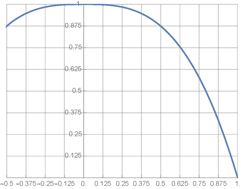
Example 1.2.4. Estimating area: \(f(x)=1-\abs{x}^3\).

Let \(f(x)=1-\val{x}^3\text{,}\) and let \(\mathcal{C}\) be the graph of \(f\text{.}\) Compute the upper and lower area estimates of the region between \(\mathcal{C}\) and the \(x\)-axis from \(x=-1/2\) to \(x=1\) by dividing the interval \([-1/2,1]\) into 4 equal subintervals. Draw block pictures of your estimates on the provided graphs.

Solution.

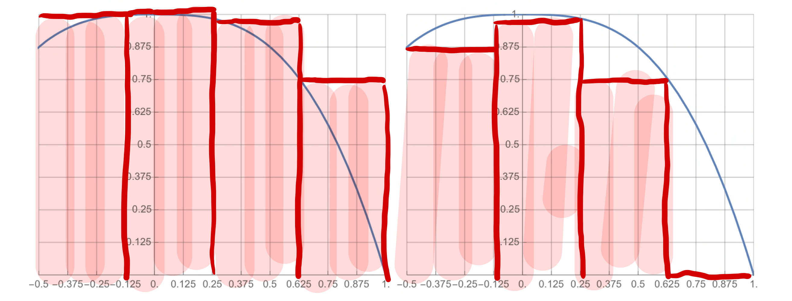
First we determine the width of the blocks: since the interval \([-1/2,1]\) has length \(3/2\text{,}\) dividing this into four equal lengths yields blocks of width \((3/2)/4=3/8=0.375\text{.}\) To pick the heights for each block, we look for the highest (resp., lowest) point in the curve over each base. Here is a diagram of the upper and lower estimates.

The corresponding area estimates are computed as follows:

\begin{align*} \text{upper estimate} \amp =f(-1/8)(3/8)+f(0)(3/8)+f(1/4)(3/8)+f(5/8)(3/8) \\ \amp = \frac{3}{8}(511/512+1+63/64+387/512)\amp (f(x)=1-\abs{x}^3)\\ \amp = 5739/2048 \approx 1.401\\ \text{lower estimate} \amp =f(-1/2)(3/8)+f(1/4)(3/8)+f(5/8)(3/8)+f(1)(3/8) \\ \amp = \frac{3}{8}(7/8+63/64+387/512+0)\amp (f(x)=1-\abs{x}^3)\\ \amp = 4017/4096 \approx 0.981 \end{align*}

Procedure 1.2.5. Estimating net change.

Suppose physical quantity \(Q=g(x)\) is a function of an input \(x\text{,}\) and that \(f(x)\) is the instantaneous rate of change of \(Q\) with respect to \(x\text{.}\)

Suppose we are only given the rate of change function \(f\) and wish to use this to estimate the net change of \(Q\) from \(x=a\) to \(x=b\text{:}\) that is, we wish to estimate \(\Delta Q=g(b)-g(a)\text{.}\) We can do so using the same method described in Procedure 1.2.2.

In this context we interpret a sample value \(r^*=f(x^*)\) as a constant rate of change over the given subinterval, in which case an individual term

\begin{equation*} f(x^*)\, \Delta x=r^* \Delta x \end{equation*}

in our sum is understood as an estimate of the net change of \(Q\) over the given subinterval, under the simplifying assumption that \(Q\) changes with constant rate of change \(r^*=f(x^*)\) over the interval.

Remark 1.2.6.

Recall that given a function \(g\text{,}\) its instantaneous rate of change with respect to \(x\) is precisely its derivative \(g'\text{.}\) This allows us to interpret Procedure 1.2.5 as a method of estimating the net change in a function \(g\) over an interval using information only about its derivative function \(f=g'\text{.}\)

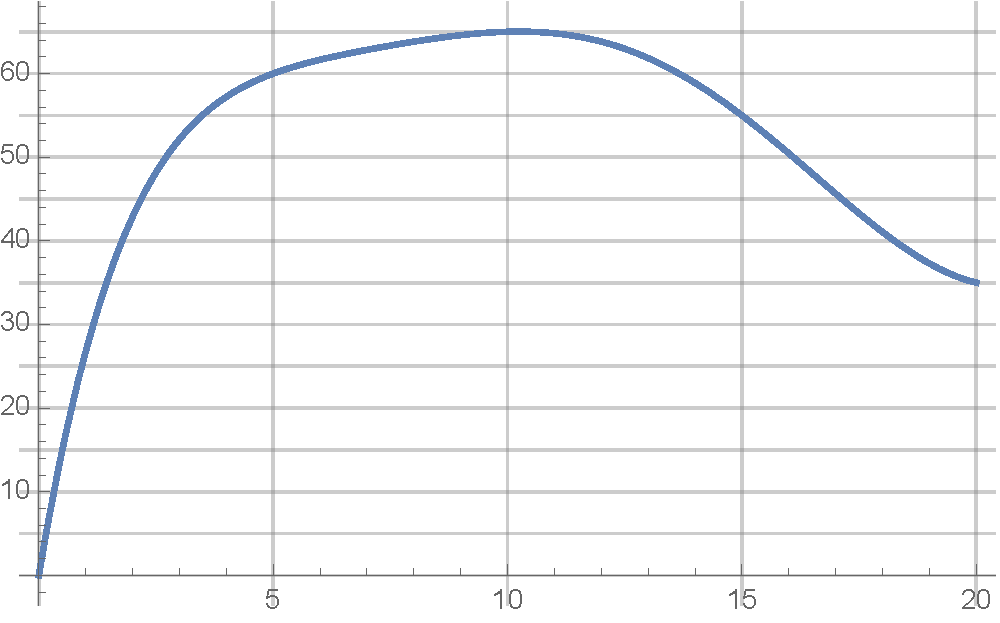
Example 1.2.7. Estimating displacement.

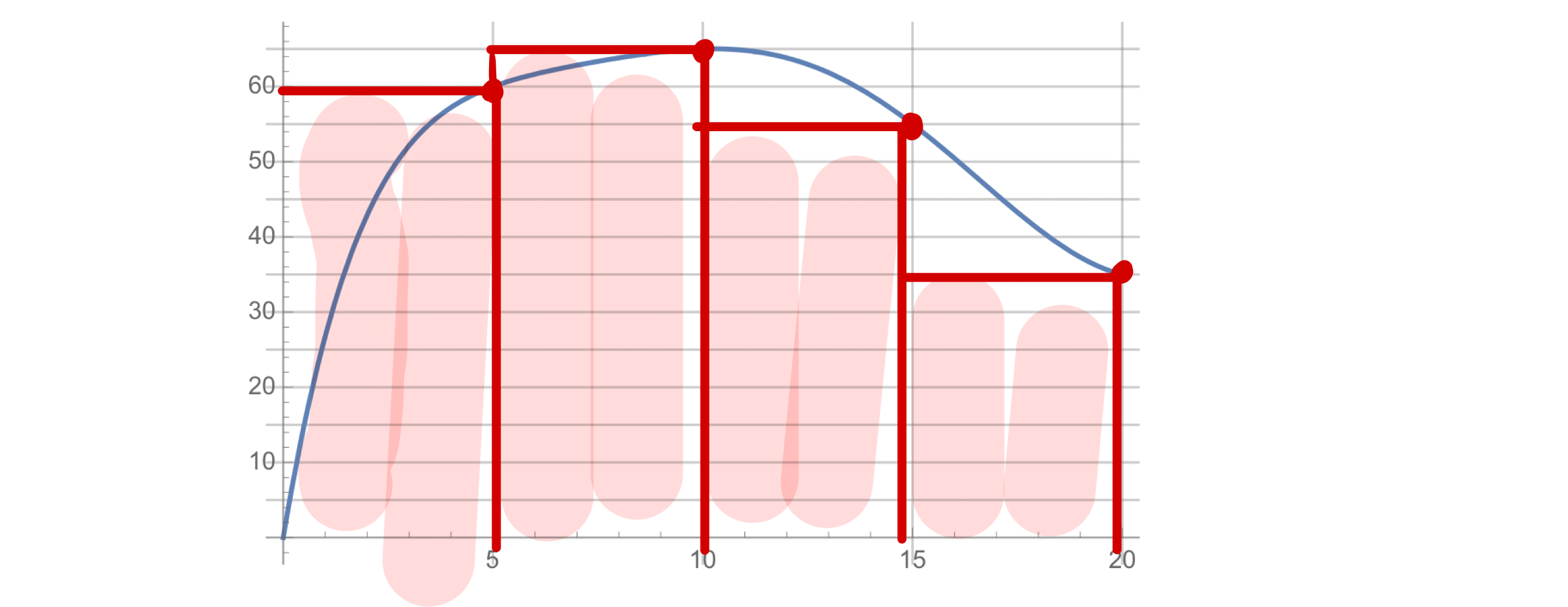
Below you find the graph of the velocity \(v(t)\) (in mph) of a driver heading due east \(t\) minutes after setting off. Compute an estimate of the area under the graph of \(v(t)\) between \(t=0\) and \(t=20\text{,}\) and explain what this estimate means physically speaking. Include units!

Solution.

First we compute an area of the region under the graph using a right sum estimate with four blocks. Here is a diagram corresponding to this estimate procedure.

Let \(B_i\) be the \(i\)-th block for each \(1\leq i\leq 4\text{,}\) and let \(A_i=\operatorname{area} B_i\text{.}\) We compute the areas \(A_i\text{,}\) and include the units of \(v\) (mph) and \(\Delta t\) (min) in our computations:

\begin{align*} A_1 \amp =v(5)\cdot 5=(60 \text{ mph}) \cdot (5 \text{ min})=(60 \text{ mph}) \cdot (1/12 \text{ min})= 5 \text{ mi}\\ A_2 \amp =v(10)\cdot 5=(65 \text{ mph}) \cdot (5 \text{ min})=(65 \text{ mph}) \cdot (1/12 \text{ min}) = 65/12 \text{ mi}\\ A_3 \amp =v(15)\cdot 5=(55 \text{ mph}) \cdot (5 \text{ min})=(55 \text{ mph}) \cdot (1/12 \text{ min}) = 55/12 \text{ mi}\\ A_4 \amp =v(20)\cdot 5=(35 \text{ mph}) \cdot (5 \text{ min})=(35 \text{ mph}) \cdot (1/12 \text{ min}) = 35/12 \text{ mi} \end{align*}

Physically speaking, the first area

\begin{equation*} A_1=v(5)\cdot 5 (=\text{velocity}\cdot \text{time})\text{,} \end{equation*}

computes the distance the driver travels eastward, had they driven at a constant speed of \(v(5)=60\) mph eastward for the full five minutes. As such, this is an approximation of the total distance the drive traveled during this segment of the drive. Similar interpretations apply to the other blocks: each area can be understood as an approximation of the distance traveled eastward during that segment of the drive. We conclude that the the driver travels approximately

\begin{equation*} \frac{1}{12}(60+65+55+35)=215/12\approx 17.9 \text{ mi} \end{equation*}

in the eastward direction.

Observe that in this example, where velocity is always positive (equivalently, the driver always travels in same direction), distance traveled over any time interval is the same thing as change in position (or displacement) over that interval. And so total distance traveled is the same thing as total change of position. This is no longer the case if the velocity function can be positive and negative. We will pick this up again later.

Prev Top Next