Substitution: spherical coordinates

Section 1.8 Substitution: spherical coordinates

As our last application of Theorem 1.6.6 we consider the spherical coordinate equations

\begin{align} x \amp = \rho\sin\phi\cos\theta\tag{1.8.1}\\ y\amp =\rho\sin\phi\sin\theta \tag{1.8.2}\\ z \amp =\rho\cos\phi \text{,}\tag{1.8.3} \end{align}

along with the auxiliary equations

\begin{align} r \amp = \sqrt{x^2+y^2}=\rho\sin\phi \tag{1.8.4}\\ \tan \phi \amp = \frac{z}{r} \text{,}\tag{1.8.5} \end{align}

derived from the diagram in Figure 1.8.1.

As before we think of these equations as defining a function

\begin{align*} G\colon \R^3 \amp\rightarrow \R^3 \\ (\rho, \phi, \theta)\amp\mapsto (\underset{x}{\underbrace{\rho\sin\phi\cos\theta}},\underset{y}{\underbrace{\rho\sin\phi\sin\theta}}, \underset{z}{\underbrace{\rho\cos\phi}}) \end{align*}

from \(\rho\phi\theta\)-space to \(xyz\)-space.

Theorem 1.8.2. Spherical change of variables.

The function

is continuously differentiable everywhere. The Jacobian of \(G\) is

\begin{equation} \frac{\partial(x,y,z)}{\partial(r,\theta,z)}=\det\begin{pmatrix} \sin\phi\cos\theta \amp\rho\cos\phi\cos\theta\amp -\rho\sin\phi\sin\theta\\ \sin\phi\sin\theta\amp \rho\cos\phi\sin\theta\amp \rho\sin\phi\cos\theta\\ \cos\phi\amp -\rho\sin\phi\amp 0 \end{pmatrix}=\rho^2\sin\phi\text{.}\tag{1.8.6} \end{equation}

Assume \(G\) is one-to-one on the interior of \(\mathcal{R}\subseteq\R^3\text{,}\) and let \(\mathcal{S}=G(\mathcal{R})\) be the image under \(G\text{.}\) If \(f\) is continuous on the interior of \(\mathcal{R}\text{,}\) then by Theorem 1.6.6 we have

\begin{align} \iiint\limits_\mathcal{S}f(x,y,z)\, dV \amp =\iiint\limits_\mathcal{R}f(\rho\sin\phi\cos\theta, \rho\sin\phi\sin\theta, \rho\cos\phi) \, \rho^2 \abs{\sin\phi}\, dV \tag{1.8.7}\\ \amp = \iiint\limits_\mathcal{R}f(\rho\sin\phi\cos\theta, \rho\sin\phi\sin\theta, \rho\cos\phi) \, \rho^2 \sin\phi\, dV \amp (\text{assuming } 0\leq \phi\leq \pi)\text{.}\tag{1.8.8} \end{align}

Procedure 1.8.3. Integrating using spherical change of variables.

When computing an integral \(\iiint\limits_Df(x,y,z)\, dV\) using a spherical change of variables, we often end up describing the corresponding region in \(\rho\phi\theta\)-space in type-B form. In this case, proceed as follows.

Sketch.
Sketch \(D\) along with its projection \(\mathcal{R}\) onto the \(xy\)-plane.
\(\rho\)-limits of integration.
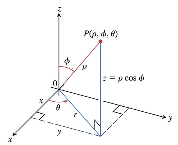
For each \(\phi\in [0,\pi]\) and \(\theta\in [0,2\pi]\text{,}\) let \(R_{\phi,\theta}\) be the ray through the origin that makes an angle of \(\phi\) with the positive \(z\)-axis, and whose projection on the \(xy\)-plane makes an angle of \(\theta\) with the positive \(x\)-axis. The \(\rho\)-values of the points where the ray \(R_{\phi,\theta}\) enters and leaves \(D\) give us our \(\rho\)-bounds \(p_1(\phi,\theta)\leq \rho\leq p_2(\phi,\theta)\text{.}\)
\(\phi\)-limits of integration.
For each \(\theta\in [0,2\pi]\text{,}\) as we let \(\phi\) vary the ray \(R_{\phi,\theta}\) sweeps through \(D\text{.}\) The \(\phi\) values \(g_1(\theta), g_2(\theta)\) of the points where the sweeping ray enters and leaves \(D\) give us our \(\phi\)-bounds \(g_1(\theta)\leq \phi\leq g_2(\theta)\text{.}\)
\(\theta\)-limits of integration.
As we let \(\theta\) vary, the ray \(L_\theta\) in the \(xy\)-plane making an angle of \(\theta\) with the positive \(x\)-axis rotates around the \(z\)-axis and sweeps across \(\mathcal{R}\text{.}\) The \(\theta\)-values \(\theta_1, \theta_2\) of the points where the sweeping ray enters and leaves \(\mathcal{R}\) give us our \(\theta\)-bounds \(\theta_1\leq \theta\leq \theta_2\text{.}\)
Integrate.
Use cylindrical substitution and Fubini's theorem to conclude

\begin{equation*} \iiint\limits_Df(x,y,z)\, dV=\int_{\theta_1}^{\theta_2}\int_{g_1(\theta)}^{g_2(\theta)}\int_{p_1(\phi,\theta)}^{p_2(\phi,\theta)}f(\rho\sin\phi\cos\theta, \rho\sin\phi\sin\theta, \rho\cos\phi)\rho^2\sin\phi\, d\rho\, d\phi\, d\theta\text{.} \end{equation*}

Remark 1.8.4. Converting to spherical coordinates.

Example 1.8.5. Average distance over a solid sphere.

Compute the average distance to the origin of points \((x,y,z)\) lying within the sphere \(x^2+y^2+z^2= R^2\text{,}\) where \(R\) is a fixed positive constant.

Solution.

Let \(D\) be the region lying within the sphere. Observe that the function in question is \(f(x,y,z)=\sqrt{x^2+y^2+z^2}\text{.}\) In spherical coordinates the solid sphere is described as

\begin{equation*} \{(\rho, \phi, \theta)\colon 0\leq \theta\leq 2\pi, 0\leq \phi\leq \pi, 0\leq \rho\leq R\}\text{.} \end{equation*}

We have

\begin{align*} \operatorname{avg}_D f \amp =\frac{1}{\operatorname{vol} D} \iiint\limits_D \sqrt{x^2+y^2+z^2}\, dV \\ \amp=\frac{3}{4\pi R^3}\int_0^{2\pi}\int_0^\pi\int_0^R\rho\cdot \rho^2\sin\phi\, d\rho\, d\phi\, d\theta \amp \text{(spher. subst.)}\\ \amp = \frac{3}{2 R^3}\pi\int_0^\pi\sin\phi\, d\phi \int_0^R\rho^3\, d\rho\\ \amp = \frac{3}{2 R^3} (-\cos\phi)\Bigr\vert_0^{\pi}\left(\frac{1}{4}\rho^4\right)\Bigr\vert_0^R\\ \amp =\frac{3}{4}R\text{.} \end{align*}

Example 1.8.6. Volume of ice cream cone.

Let \(D\) be the region lying above the cone \(z=\sqrt{x^2+y^2}\) and within the sphere \(x^2+y^2+(z-R)^2=R^2\text{,}\) where \(R\) is a fixed positive constant. Compute the volume of \(D\) as a triple integral.

Solution.

First we convert the equation \(z=\sqrt{x^2+y^2}\) defining the cone into spherical coordinates with the help of the auxiliary equations (1.8.4)–(1.8.5):

\begin{align*} z=\sqrt{x^2+y^2} \amp \iff \frac{z}{r}=1\\ \amp\iff \tan\phi=1 \\ \amp \iff \phi=\pi/4\text{.} \end{align*}

We see that for a point to lie within the cone \(z=\sqrt{x^2+y^2}\) we need \(0\leq \phi\leq \pi/4\text{.}\) Next, we describe the given sphere in spherical coordinates:

\begin{align*} x^2+y^2+(z-R)^2\leq R^2\amp\iff x^2+y^2+z^2-2Rz\leq 0 \\ \amp\iff \rho^2\leq 2R\rho\cos\phi \\ \amp \iff \rho\leq 2R\cos\phi \text{ or } \rho=0\\ \amp \iff 0\leq \rho\leq 2R\cos\phi\text{.} \end{align*}

Thus the spherical description of \(D\) is

\begin{equation*} \{(\rho, \phi,\theta)\colon 0\leq \theta\leq 2\pi, 0\leq \phi\leq \pi/4, 0\leq \rho\leq 2R\cos\phi\}\text{.} \end{equation*}

Now compute

\begin{align*} \operatorname{vol} D \amp=\iiint\limits_D 1\, dV \\ \amp = \int_0^{2\pi}\int_0^{\pi/4}\int_0^{2R\cos\phi}\rho^2\sin\phi\, d\rho\, d\phi\, d\theta \amp \text{(spher. coord.)}\\ \amp =2\pi\int_0^{\pi/4}\frac{1}{3}\sin\phi(2R\cos\phi)^3\, d\phi \\ \amp =\frac{16}{3}\pi R^3\int_0^{\pi/4}\sin\phi\cos^3\phi\, d\phi\\ \amp =\frac{16}{3}\pi R^3\left(-\frac{1}{4}\cos^4\phi\right)\Bigr\vert_0^{\pi/4}\\ \amp =\frac{16}{12}\pi R^3(1-(\sqrt{2}/2)^4)\\ \amp =\frac{16}{12}\pi R^3(3/4)\\ \amp =\pi R^3\text{.} \end{align*}

Math 230-2: Kursobjekt

Search Results: