Section 1.7 Substitution: polar and cylindrical coordinates
Theorems 1.7.3–1.7.9 result from applying Theorem 1.6.6 to particular transformations, called the polar and cylindrical transformations:
Subsection 1.7.1 Polar transformation
We will think of the polar coordinate equations
as defining a function
from one copy of \(\R^2\text{,}\) called the \(r\theta\)-plane, to another, called the \(xy\)-plane. Earlier in your calculus career you learned to translate back and forth between polar equations and Cartesian (or rectangular) ones. We will now think of these translations as evaluations of the function \(G\) or its inverse to regions of the \(r\theta\)- or \(xy\)-plane. For example, \(G\) takes the rectangle
lying in the \(r\theta\)-plane, and maps it to the set of all points in the \(xy\)-plane lying between the circles of radius \(r=r_1\) and \(r=r_2\text{,}\) centered at the origin, and between the two rays obtained by rotating the positive \(x\)-axis by an angle of \(\theta=\theta_1\) and \(\theta=\theta_2\text{,}\) respectively. 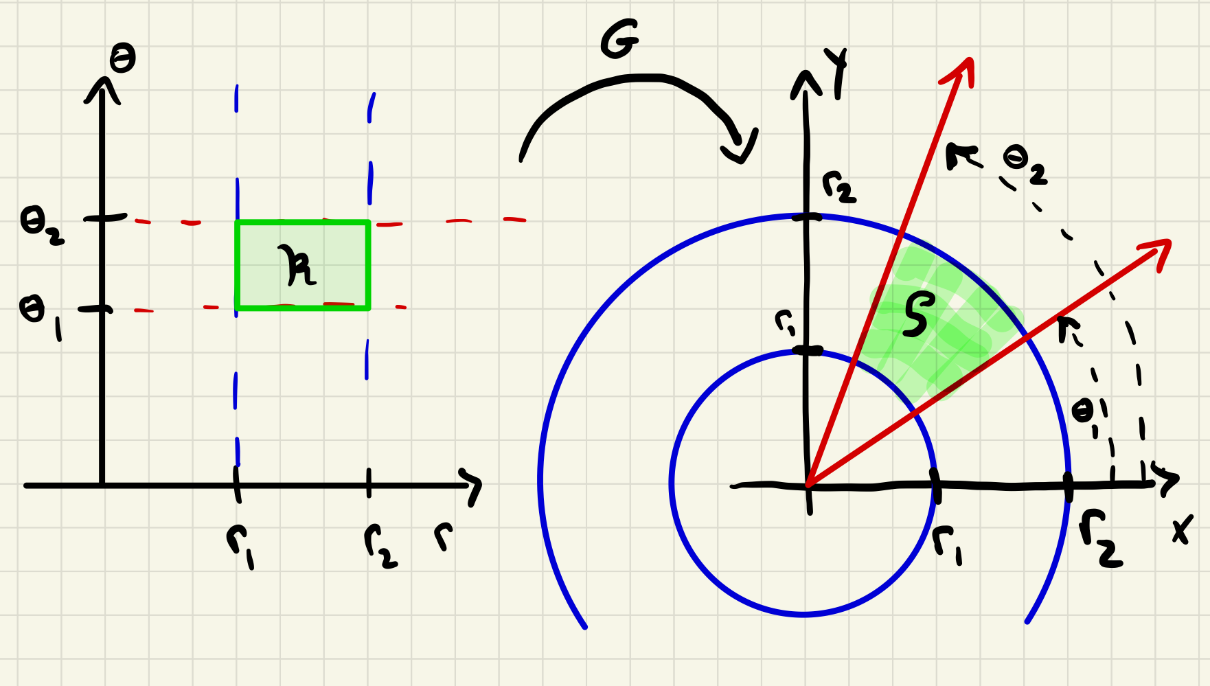
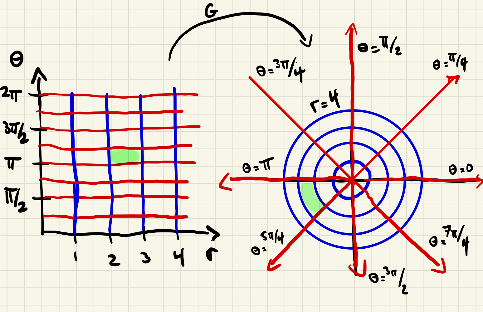
It is easy to see that \(G\) is continuously differentiable, and hence is a candidate for an application of Theorem 1.6.6. The only thing we need to be careful about is restricting ourselves to regions \(\mathcal{R}\) where \(G\) is one-to-one, and hence defines a transformation.
Theorem 1.7.3. Polar change of variables.
The function
Remark 1.7.4. Polar transformation.
It is not difficult to show that
It follows that the polar function \(G(r,\theta)=(r\cos\theta, r\sin\theta)\) is one-to-one on a given set as long as it doesn't contain pairs of points satisfying one of the conditions in (1.7.4). Below you find two common types of sets where \(G\) is one-to-one:
Observe that \(r\) values are allowed to be positive or negative in the set \(Y\text{,}\) and so the range of \(\theta\) needs to be restricted accordingly.
Example 1.7.5. Area between limaçon and circle.
Let \(\mathcal{S}\subseteq \R^2\) be the region outside the circle of radius 2, centered at the origin, and inside the limaçon with polar equation
Compute the area of \(\mathcal{S}\text{.}\)
The \(r\theta\)-coordinates of points in \(\mathcal{S}\) satisfy \(r=1+2\sin\theta\geq 2\text{.}\) A little algebra shows this implies \(\pi/6\leq \theta\leq 5\pi/6\text{.}\) Thus the polar transformation \(G(r,\theta)=(r\cos\theta, r\sin\theta)\) maps the \(r\theta\)-region
onto \(\mathcal{S}\text{.}\) Using Theorem 1.7.3, we have
Example 1.7.6. Average value over semicircle.
Compute the average value of \(f(x,y)=x\) over the semicircular region
where \(R\in \R\) is a fixed constant.
The half-disk \(\mathcal{R}\) corresponds to the the region
in the \(r\theta\)-plane via the polar transformation \(G(r,\theta)=(r\cos\theta,r\sin\theta)\text{.}\) We have
Subsection 1.7.2 Cylindrical transformation
Our discussion in Subsection 1.7.1 generalizes easily to cylindrical coordinates:
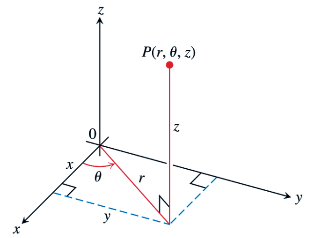
from \(r\theta z\)-space to \(xyz\)-space. Recalling some of our translation exercises from cylindrical to and from Cartesian coordinates we see that \(G\) maps the box
lying in \(r\theta z\)-space, to a certain region of \(xyz\)-space trapped between two vertical circular cylinders of radius \(r_1\) and \(r_2\text{.}\) 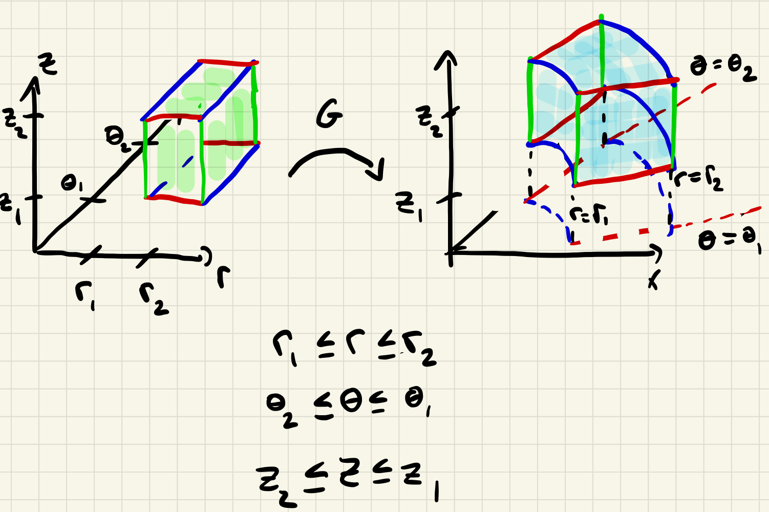
Theorem 1.7.9. Cylindrical change of variables.
The function
Procedure 1.7.10. Integrating using cylindrical change of variables.
When computing an integral \(\iiint\limits_Df(x,y,z)\, dV\) using a cylindrical change of variables, we often end up describing the corresponding region in \(r\theta z\)-space in type-A form. In this case, proceed as follows.
-
Sketch.
Sketch \(D\) along with its projection \(\mathcal{R}\) onto the \(xy\)-plane.
-
\(z\)-limits of integration.
For each point \((r,\theta,0)\in \mathcal{R}\) visualize the line parallel to the \(z\)-axis passing through it, and observe where this line enters and exits \(D\text{.}\) The \(z\)-values \(p_1(r,\theta), p_2(r,\theta)\) give us our \(z\)-bounds \(p_1(r,\theta)\leq z\leq p_2(r,\theta)\text{.}\)
-
\(r\)-limits of integration.
For each \(\theta\in [0,2\pi]\text{,}\) imagine the ray \(L_\theta\) in the \(xy\)-plane that makes an angle of \(\theta\) with the positive \(x\)-axis. The \(r\)-values \(g_1(\theta), g_2(\theta)\) of the points where \(L_\theta\) enters and leaves \(\mathcal{R}\) give us our \(r\)-bounds \(g_1(\theta)\leq r\leq g_2(\theta)\text{.}\)
-
\(\theta\)-limits of integration.
As we let \(\theta\) vary, the ray \(L_\theta\) rotates around the \(z\)-axis and sweeps across \(\mathcal{R}\text{.}\) The \(theta\)-values \(\theta_1, \theta_2\) of the points where the sweeping ray enters and leaves \(\mathcal{R}\) give us our \(\theta\)-bounds \(\theta_1\leq \theta\leq \theta_2\text{.}\)
-
Integrate.
Use cylindrical substitution and Fubini's theorem to conclude
\begin{equation*} \iiint\limits_Df(x,y,z)\, dV=\int_{\theta_1}^{\theta_2}\int_{g_1(\theta)}^{g_2(\theta)}\int_{p_1(r,\theta)}^{p_2(r,\theta)}f(r\cos\theta, r\sin\theta, z)\, r\, dz\, dr\, d\theta\text{.} \end{equation*}
Example 1.7.11. Volume of sphere: cylindrical coordinates.
Consider the solid spherical ball
where \(R\in \R\) is a fixed constant. Compute the volume of \(\mathcal{S}\) using cylindrical coordinates.
The projection of \(\mathcal{S}\) onto the \(xy\)-plane is the disk \(x^2+y^2\leq R^2\text{,,}\) which is described in cylindrical coordinates as \(0\leq \theta\leq 2\pi, 0\leq r\leq R\text{.}\) Next, looking at the vertical line passing through a point \((r,\theta,0)\text{,}\) we see we enter and leave \(\mathcal{S}\) at the lower and upper surfaces of the sphere. In cylindrical coordinates the defining equation \(x^2+y^2+z^2=R^2\) becomes \(r^2+z^2=R^2\text{,}\) and thus the lower and upper surfaces of the sphere have cylindrical equations \(z=-\sqrt{R^2-r^2}\) and \(z=\sqrt{R^2-r^2}\text{,}\) repsectively. We conclude that the cylindrical description of \(\mathcal{S}\) is
Finally, we compute
We've just derived the volume formula for the sphere of radius \(R\text{!}\)
Example 1.7.12. Average value over hemisphere: cylindrical coordinates.
Consider the solid hemisphere
where \(R\in \R\) is a fixed constant. Find the average height (distance to \(xy\)-plane) of points in \(\mathcal{S}\text{.}\)
First observe that the function in question is just \(f(x,y,z)=z\text{.}\) The cylindrical description of \(\mathcal{S}\) is similar to the previous example, except now \(z\)-values are bounded below by zero:
Now compute
