Section 2.1 Line integrals of scalar functions
Subsection 2.1.1 Curve parametrizations
Definition 2.1.1. Curve parametrization.
A curve parametrization (or path) is a continuous function
where \(I\subseteq \R\) is an interval. The functions \(x_i(t)\) defining \(\boldr\) are called component functions.
The setWhen \(n=2\) we call \(\boldr\colon I\rightarrow \R^2\) a parametrized planar curve; when \(n=3\) we call \(\boldr\colon I\rightarrow \R^3\) a parametrized space curve.
A path \(\boldr(t)=(x_1(t),x_2(t),\dots, x_n(t))\) is smooth on an interval \(I\) if the functions \(x_i(t)\) are continuously differentiable on \(I\) and \(\boldr'(t)\ne \boldzero\) for all \(t\in I\text{.}\)
Remark 2.1.2.
Qualitatively, a parametrization \(\boldr\colon I\rightarrow \R^n\) takes as an input a real number \(t\text{,}\) and returns as an output a tuple \(\boldr(t)=(x_1(t),x_2(t),\dots, x_n(t))\text{.}\) This is an example of what we call a vector-valued function, as the output of the function is not a scalar, but a tuple (pair if \(n=2\text{,}\) triple if \(n=3\)).
Geometrically, we can think of a tuple either as a point \(P\) in \(\R^n\text{,}\) or as an \(n\)-vector \(\boldv=\langle v_1,v_2,\dots, v_n\rangle\text{.}\) When visualizing a path \(\boldr\) and its outputs, we will make use of both interpretations. The table below recalls some standard interpretations of \(\boldr(t)\) and \(\boldr'(t)\) along these lines. For simplicity, we assume \(n=3\text{.}\)
Remark 2.1.3. Parametrizations you should know.
-
Line through \(P=(a,b,c)\) with direction vector \(\boldv=(v_1,v_2,v_3)\text{:}\)
\begin{equation*} \boldr(t)=(a,b,c)+t\boldv=(a+tv_1,b+tv_2,c+tv_3)\text{.} \end{equation*} -
Line segment between points \(P=(a,b,c), Q=(d,e,f)\text{:}\)
\begin{equation*} \boldr(t)=P+t(Q-P)=(1-t)P+tQ, \ 0\leq t\leq 1\text{.} \end{equation*} -
Circle of radius \(R\) centered at \((a,b)\text{:}\)
\begin{equation*} \boldr(t)=(a,b)+R(\cos t, \sin t)=(a+R\cos t, b+R\sin t), \ 0\leq t\leq 2\pi\text{.} \end{equation*} -
Ellipse \(\frac{x^2}{a^2}+\frac{y^2}{b^2}=1\text{:}\)
\begin{equation*} \boldr(t)=(a\cos t, b\sin t), \ 0\leq t\leq 2\pi\text{.} \end{equation*} -
Helix of radius \(R\) along a given coordinate axis in \(3\)-space. Example:
\begin{equation*} \boldr(t)=(R\cos t, t, R\sin t)\text{.} \end{equation*}
Sage example 2.1.1. Parametrized curves.
parametric_plot (\(n=2\)) or parametric_plot3d (\(n=3\)). The cell below graphs parametrizations of circles confined in various planes in \(3\)-space. The next cell illustrates line parametrizations. Try plotting the remaining examples of parametrizations from Remark 2.1.3 in the cell below. If using a plane curve parametrization, delete the # in front of parametric_plot(r(t), (t,a,b)); if using a space curve parametrization, delete the # in front of parametric_plot3d(r(t), (t,a,b)). Subsection 2.1.2 Line integrals of a scalar function
Definition 2.1.4. Line integral of scalar function.
Let \(\boldr\colon [a,b]\rightarrow \R^3\) be a parametrization of the curve \(\mathcal{C}\text{,}\) and let \(f(x,y,z)\) be a scalar function defined on \(\mathcal{C}\text{.}\)
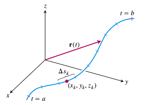
Let \(P=\boldr(a)\) and \(Q=\boldr(b)\) be the start and end points of the path \(\boldr\text{.}\) A pointed partition of of the path \(\boldr\) along \(\mathcal{C}\) is the sequence of points \(P=\boldr(a), P_1=\boldr(t_1), P_2=\boldr(t_2), \dots, Q=\boldr(b)\) corresponding to a partition \(a=t_0 < t_1< t_2\dots < t_n=b \) of the interval \([a,b]\text{,}\) along with a selection of points \((x_k,y_k,z_k)\) lying in the \(k\)-th segment of the partitioned path. We define \(\Delta s_k\) to be the arc length of the curve segment between \(P_{k-1}\) and \(P_k\text{.}\)
The line integral of \(f\) over \(\mathcal{C}\text{,}\) denoted \(\int\limits_\mathcal{C}f(x,y,z)\, ds\text{,}\) is defined as
where the limit is understood to be taken over any sequence of pointed partitions \(P_n\) of \(\mathcal{C}\) into \(n\) curve segments, provided this limit exists and is independent of our choice of partitions.

As with double and triple integrals, the limit definition of line integrals is useful for interpretation purposes, but not so convenient for computation. The following theorem is the essential tool we will use for computing line integrals.
Theorem 2.1.6. Scalar line integrals.
Let \(\boldr\colon [a,b]\rightarrow \R^n\) be a parametrization of the curve \(\mathcal{C}\subseteq \R^n\text{,}\) and let \(f(x_1,x_2,\dots, x_n)\) be a scalar function defined on \(\mathcal{C}\text{.}\) If (a) \(\boldr\) is smooth on \([a,b]\) and (b) \(f(x,y,z)\) is continuous on \(\mathcal{C}\text{,}\) then
Remark 2.1.7. Independence of parametrization.
Do different parametrizations of the same curve \(\mathcal{C}\) lead to different line integrals of a function \(f\text{?}\) Absolutely! Consider
Both parametrize the unit circle \(\mathcal{C}\colon x^2+y^2=1\text{.}\) However, the integral of the constant function \(f(x,y)=1\) over \(\boldr(t)\) yields \(2\pi\) (the arc length of \(\mathcal{C}\)), while the integral of \(\bolds(t)\) yields \(4\pi\) (twice the arc length of \(\mathcal{C}\)). This makes sense, since \(\bolds(t)\) traverses \(\mathcal{C}\) twice!
On the other hand, you can show that if the parametrizations \(\boldr\) and \(\bolds\) are smooth and one-to-one on \([a,b]\text{,}\) except possibly at the endpoints, then indeed the two line integrals will be equal. Thus, we say the line integral is independent of your choice of smooth, one-to-one parametrization.
Theorem 2.1.8. Interpretations.
Assume \(\boldr\colon [a,b]\rightarrow \R^n\) is a smooth parametrization of \(\mathcal{C}\) and that \(\boldr\) is one-to-one on \([a,b]\text{,}\) except potentially at the endpoints (i.e., “\(\boldr\) traverses \(\mathcal{C}\) exactly once”).
The line integral \(\int_\mathcal{C} 1\, ds\) computes the arc length of \(\mathcal{C}\) between \(P=\boldr(a)\) and \(Q=\boldr(b)\text{.}\)
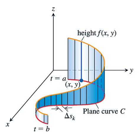
If \(n=2\) and \(f(x,y)\geq 0\) is continuous on \(\mathcal{C}\text{,}\) then \(\int_\mathcal{C}f(x,y)\, ds\) computes the area of the “curtain” over \(\mathcal{C}\) with heights given by \(f(x,y)\text{.}\)
If \(\delta(x_1,x_2,\dots, x_n)\geq 0\) is a continuous mass density on \(\mathcal{C}\text{,}\) where \(\mathcal{C}\) is treated as an infinitely thin wire, then \(\int_\mathcal{C}\delta(x_1,x_2,\dots, x_n)\, ds\) computes the mass of \(\mathcal{C}\text{.}\)

Theorem 2.1.10. Piecewise smooth line integral.
Assume the parametrized curve \(\mathcal{C}\) is a union of smoothly parametrized curves \(\mathcal{C}_1, \mathcal{C}_2,\dots, \mathcal{C}_r\text{.}\) If \(f\) is continuous on \(\mathcal{C}\text{,}\) then
Example 2.1.11. Line integral of helix.
Let \(\mathcal{C}\) be the helix with parametrization \(\colon \boldr(t)=(2\sin t, t, 2\cos t)\text{,}\) \(0\leq t\leq \pi\text{,}\) and let \(f(x,y,z)=x^2+y^2+z^2\text{.}\) Compute \(\int\limits_\mathcal{C}f(x,y,z)\, ds\text{.}\)
Assemble the ingredients:
Now compute
Example 2.1.12. Area of a curtain.
Compute the area of the curtain over the curve \(x=y^2\) between the points \(P=(1,-1)\) and \(Q=(4,2)\text{,}\) with height function given by \(f(x,y)=\sqrt{x}+\abs{y}\)
The segment of the curve in question has parametrization \(\boldr(t)=(t^2,t)\text{,}\) \(-1\leq t\leq 2 \text{.}\) (Observe that \(\boldr(-1)=(1,-1)=P, \boldr(2)=(4,2)=Q\text{.}\)) According to Theorem 2.1.8 we have
Example 2.1.13. Mass of wire.
Let \(P=(1,1,0), Q=(1,2,2), R=(2,2,5)\text{,}\) and let \(\mathcal{C}\) be the polygonal wire connecting \(P\) to \(Q\) and \(Q\) to \(R\text{.}\) Compute the mass \(M\) of the wire assuming its density function is given by \(\delta(x,y,z)=x(y+z)\text{.}\)
The path in question is piecewise smooth, allowing us to use Theorem 2.1.10. We use the straight line parametrizations
and assemble some ingredients
Lastly we compute
Sage example 2.1.2. Scalar line integral.
The basic ingredients of a line integral are an expression \(\boldr(t)\) defining a parametrized curve, the domain \([a,b]\) of \(\boldr\text{,}\) and the function \(f\) we are integrating. You can see how the Sage cell below assembles these basic ingredients, along with the further ingredients \(\boldr'(t)\) and \(\abs{\boldr'(t)}\text{,}\) before computing the line integral using Theorem 2.1.6. Note how we use the vector() command to create vector objects. This is essential for doing any further vector operations: e.g., dot product, norm, etc..
